Download
1 / 78
810 likes | 1.55k Views
CHAPTER 8 Hashing. Instructors: C. Y. Tang and J. S. Roger Jang. All the material are integrated from the textbook "Fundamentals of Data Structures in C" and some supplement from the slides of Prof. Hsin-Hsi Chen (NTU). Concept of Hashing.

E N D
CHAPTER 8 Hashing Instructors: C. Y. Tang and J. S. Roger Jang All the material are integrated from the textbook "Fundamentals of Data Structures in C" and some supplement from the slides of Prof. Hsin-Hsi Chen (NTU).
Concept of Hashing In CS, a hash table, or a hash map, is a data structure that associates keys (names) with values (attributes). Look-Up Table Dictionary Cache Extended Array
Example A small phone book as a hash table. (Figure is from Wikipedia)
Dictionaries Collection of pairs. (key, value) Each pair has a unique key. Operations. Get(theKey) Delete(theKey) Insert(theKey, theValue)
Just An Idea Hash table : Collection of pairs, Lookup function (Hash function) Hash tables are often used to implement associative arrays, Worst-case time for Get, Insert, and Delete is O(size). Expected time is O(1).
Origins of the Term The term "hash" comes by way of analogy with its standard meaning in the physical world, to "chop and mix.” D. Knuth notes that Hans Peter Luhn of IBM appears to have been the first to use the concept, in a memo dated January 1953; the term hash came into use some ten years later.
Search vs. Hashing • Search tree methods: key comparisons • Time complexity: O(size) or O(log n) • Hashing methods: hash functions • Expected time: O(1) • Types • Static hashing (section 8.2) • Dynamic hashing (section 8.3)
Static Hashing • Key-value pairs are stored in a fixed size table called a hash table. • A hash table is partitioned into many buckets. • Each bucket has many slots. • Each slot holds one record. • A hash function f(x) transforms the identifier (key) into an address in the hash table
Hash table s slots 0 1 s-1 0 1 b buckets b-1
Data Structure for Hash Table #define MAX_CHAR 10 #define TABLE_SIZE 13 typedef struct { char key[MAX_CHAR]; /* other fields */ } element; element hash_table[TABLE_SIZE];
Other Extensions Hash List and Hash Tree (Figure is from Wikipedia)
Formal Definition Hash Function In addition, one-to-one / onto
The Scheme Figure is from Data Structures and Program Design In C++, 1999 Prentice-Hall, Inc.
Ideal Hashing Uses an array table[0:b-1]. Each position of this array is a bucket. A bucket can normally hold only one dictionary pair. Uses a hash function f thatconverts each key k into an index in the range [0, b-1]. Every dictionary pair (key, element) is stored in its home bucket table[f[key]].
Example Pairs are: (22,a),(33,c),(3,d),(73,e),(85,f). Hash table is table[0:7], b = 8. Hash function is key (mod 11).
What Can Go Wrong? Where does (26,g) go? Keys that have the same home bucket are synonyms. 22 and 26 are synonyms with respect to the hash function that is in use. The bucket for (26,g) is already occupied.
Some Issues Choice of hash function. Really tricky! To avoid collision (two different pairs are in the same the same bucket.) Size (number of buckets) of hash table. Overflow handling method. Overflow: there is no space in the bucket for the new pair.
Example (fig 8.1) synonyms synonyms: char, ceil, clock, ctime synonyms overflow
Choice of Hash Function Requirements easy to compute minimal number of collisions If a hashing function groups key values together, this is called clustering of the keys. A good hashing function distributes the key values uniformly throughout the range.
Some hash functions Middle of square H(x):= return middle digits of x^2 Division H(x):= return x % k Multiplicative: H(x):= return the first few digits of the fractional part of x*k, where k is a fraction. advocated by D. Knuth in TAOCP vol. III.
Some hash functions II Folding: Partition the identifier x into several parts, and add the parts together to obtain the hash address e.g. x=12320324111220; partition x into 123,203,241,112,20; then return the address 123+203+241+112+20=699 Shift folding vs. folding at the boundaries Digitanalysis: If all the keys have been known in advance, then we could delete the digits of keys having the most skewed distributions, and use the rest digits as hash address.
Hashing By Division Domain is all integers. For a hash table of size b, the number of integers that get hashed into bucket i is approximately 232/b. The division method results in a uniform hash function that maps approximately the same number of keys into each bucket.
Hashing By Division II In practice, keys tend to be correlated. If divisor is an even number, odd integers hash into odd home buckets and even integers into even home buckets. 20%14 = 6, 30%14 = 2, 8%14 = 8 15%14 = 1, 3%14 = 3, 23%14 = 9 divisor is an odd number, odd (even) integers may hash into any home. 20%15 = 5, 30%15 = 0, 8%15 = 8 15%15 = 0, 3%15 = 3, 23%15 = 8
Hashing By Division III Similar biased distribution of home buckets is seen in practice, when the divisor is a multiple of prime numbers such as 3, 5, 7, … The effect of each prime divisor p of b decreases as p gets larger. Ideally, choose large prime number b. Alternatively, choose b so that it has no prime factors smaller than 20.
Hash Algorithm via Division int hash(char *key) { return (transform(key) % TABLE_SIZE); } void init_table(element ht[]) { int i; for (i=0; i<TABLE_SIZE; i++) ht[i].key[0]=NULL; } int transform(char *key) { int number=0; while (*key) number += *key++; return number; }
Criterion of Hash Table The key density (or identifier density) of a hash table is the ratio n/T n is the number of keys in the table T is the number of distinct possible keys The loading density or loading factor of a hash table is = n/(sb) s is the number of slots b is the number of buckets
Example synonyms synonyms: char, ceil, clock, ctime synonyms overflow b=26, s=2, n=10, =10/52=0.19, f(x)=the first char of x
Overflow Handling An overflow occurs when the home bucket for a new pair (key, element) is full. We may handle overflows by: Search the hash table in some systematic fashion for a bucket that is not full. Linear probing (linear open addressing). Quadratic probing. Random probing. Eliminate overflows by permitting each bucket to keep a list of all pairs for which it is the home bucket. Array linear list. Chain.
Linear probing (linear open addressing) Open addressing ensures that all elements are stored directly into the hash table, thus it attempts to resolve collisions using various methods. Linear Probing resolves collisions by placing the data into the next open slot in the table.
Linear Probing – Get And Insert divisor = b (number of buckets) = 17. Home bucket = key % 17. 0 4 8 12 16 34 0 45 6 23 7 28 12 29 11 30 33 • Insert pairs whose keys are 6, 12, 34, 29, 28, 11, 23, 7, 0, 33, 30, 45
Linear Probing – Delete Delete(0) 0 4 8 12 16 34 0 45 6 23 7 28 12 29 11 30 33 0 4 8 12 16 34 45 6 23 7 28 12 29 11 30 33 0 4 8 12 16 34 45 6 23 7 28 12 29 11 30 33 • Search cluster for pair (if any) to fill vacated bucket.
Linear Probing – Delete(34) Search cluster for pair (if any) to fill vacated bucket. 0 4 8 12 16 34 0 45 6 23 7 28 12 29 11 30 33 0 4 8 12 16 0 45 6 23 7 28 12 29 11 30 33 0 4 8 12 16 0 45 6 23 7 28 12 29 11 30 33 0 4 8 12 16 0 45 6 23 7 28 12 29 11 30 33
Linear Probing – Delete(29) Search cluster for pair (if any) to fill vacated bucket. 0 4 8 12 16 34 0 45 6 23 7 28 12 29 11 30 33 0 4 8 12 16 34 0 45 6 23 7 28 12 11 30 33 0 4 8 12 16 34 0 45 6 23 7 28 12 11 30 33 0 4 8 12 16 34 0 45 6 23 7 28 12 11 30 33 0 4 8 12 16 34 0 6 23 7 28 12 11 30 45 33
Performance Of Linear Probing Worst-case find/insert/erase time is (n), where n is the number of pairs in the table. This happens when all pairs are in the same cluster. 0 4 8 12 16 34 0 45 6 23 7 28 12 29 11 30 33
Expected Performance = loading density = (number of pairs)/b. = 12/17. Sn = expected number of buckets examined in a successful search when n is large Un = expected number of buckets examined in a unsuccessful search when n is large Time to put and remove is governed by Un. 0 4 8 12 16 34 0 45 6 23 7 28 12 29 11 30 33
Expected Performance Sn ~ ½(1 + 1/(1 – )) Un ~ ½(1 + 1/(1 – )2) Note that 0 <= <= 1. The proof refers to D. Knuth’s TAOCP vol. III <= 0.75 is recommended.
Linear Probing (program 8.3) void linear_insert(element item, element ht[]){ int i, hash_value; i = hash_value = hash(item.key); while(strlen(ht[i].key)) { if (!strcmp(ht[i].key, item.key)) { fprintf(stderr, “Duplicate entry\n”); exit(1); } i = (i+1)%TABLE_SIZE; if (i == hash_value) { fprintf(stderr, “The table is full\n”); exit(1); } } ht[i] = item; }
Problem of Linear Probing Identifiers tend to cluster together Adjacent cluster tend to coalesce Increase the search time
Coalesce Phenomenon Average number of buckets examined is 41/11=3.73
Quadratic Probing Linear probing searches buckets (H(x)+i2)%b Quadratic probing uses a quadratic function of i as the increment Examine buckets H(x), (H(x)+i2)%b, (H(x)-i2)%b, for 1<=i<=(b-1)/2 b is a prime number of the form 4j+3, j is an integer
Random Probing Random Probing works incorporating with random numbers. H(x):= (H’(x) + S[i]) % b S[i] is a table with size b-1 S[i] is a random permuation of integers [1,b-1].
Rehashing Rehashing: Try H1, H2, …, Hm in sequence if collision occurs. Here Hi is a hash function. Double hashing is one of the best methods for dealing with collisions. If the slot is full, then a second hash function is calculated and combined with the first hash function. H(k, i) = (H1(k) + i H2(k) ) % m
Summary: Hash Table Design Performance requirements are given, determine maximum permissible loading density. Hash functions must usually be custom-designed for the kind of keys used for accessing the hash table. We want a successful search to make no more than 10 comparisons (expected). Sn ~ ½(1 + 1/(1 – )) <= 18/19
Summary: Hash Table Design II We want an unsuccessful search to make no more than 13 comparisons (expected). Un ~ ½(1 + 1/(1 – )2) <= 4/5 So <= min{18/19, 4/5} = 4/5.
Summary: Hash Table Design III Dynamic resizing of table. Whenever loading density exceeds threshold (4/5 in our example), rehash into a table of approximately twice the current size. Fixed table size. Loading density <= 4/5 => b >= 5/4*1000 = 1250. Pick b (equal to divisor) to be a prime number or an odd number with no prime divisors smaller than 20.
Data Structure for Chaining #define MAX_CHAR 10 #define TABLE_SIZE 13 #define IS_FULL(ptr) (!(ptr)) typedef struct { char key[MAX_CHAR]; /* other fields */ } element; typedef struct list *list_pointer; typedef struct list { element item; list_pointer link; }; list_pointer hash_table[TABLE_SIZE]; The idea of Chaining is to combine the linked list and hash table to solve the overflow problem.
Sorted Chains [0] 0 34 [4] 6 23 7 [8] 11 28 45 [12] 12 29 30 33 [16] • Put in pairs whose keys are 6, 12, 34, 29, 28, 11, 23, 7, 0, 33, 30, 45 • Bucket = key % 17.
Expected Performance Note that >= 0. Expected chain length is . Sn ~ 1 + /2. Un ~ Refer to the theorem 8.1 of textbook, and refer to D. Knuth’s TAOCP vol. III for the proof.