Download
1 / 25
250 likes | 390 Views
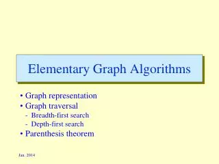
Elementary Graph Algorithms. CONTENTS Complexity Analysis (Section 3.2) Search Algorithms (Section 3.4) Topological Sorting (Section 3.4) Flow Decomposition (Section 3.5). Complexity Analysis. How to judge the goodness of an algorithm? How economically it uses the computing resources:

E N D
Elementary Graph Algorithms CONTENTS • Complexity Analysis (Section 3.2) • Search Algorithms (Section 3.4) • Topological Sorting (Section 3.4) • Flow Decomposition (Section 3.5)
Complexity Analysis • How to judge the goodness of an algorithm? • How economically it uses the computing resources: • Time efficiency • Space efficiency • Time is more crucial in practice. • How to judge the time requirement of an algorithm?
Two Type of Analysis • Empirical Analysis • Implementation dependent • Often inconclusive • Too expensive and time-consuming • Worst-Case Analysis • Obtain upper bounds on the number of steps • Often easy to perform • Mostly conclusive • Bad examples determine the performance • Most popular
Worst-Case Analysis • This type of analysis determines an upper bound on the number of steps as a function of the problem size. • The size of a problem is the number of bits required to state the problem. • The size of a network problem is a function of n, m, log C, and log U, where C denotes largest cost and U denotes the largest capacity. • If each piece of data (cost and capacity) fits into a single word, then the size of a network problem is a function of n and m. • The worst-case analysis for a network optimization algorithm determines an upper bound on the number of steps as a function of n, m, log C, and log U.
Big O Notation • Estimate the number of steps required to execute the following program: for i : = 1 to n do for j : = 1 to n do cij : = aij + bij; • The precise number of steps is implementation dependent and is very difficult to count. • MORALE: • Ignore the constants • Count each operation as one step • Consider the most dominant term when problem size becomes sufficient large
Order Notation • An algorithm is said to run in O(f(n)) time if for some numbers c and n0, the time taken by the algorithm is at most cf(n) for all n n0. • Polynomial Time Algorithms • Examples: O(n2), O(nm), O(m + n log n), O(m log C). • Exponential Time Algorithms • Examples: O(2n), O(n!) • Pseudo-Polynomial Time Algorithms • Examples: O(m+nC).
Big and Big Notation • An algorithm is said to run in (f(n)) time if for some numbers c’ and n0 and for all n n0, the algorithm takes at least cf(n) time for some problem instances. • Whereas Big O notation gives an upper bound on the running time of an algorithm, Big notation gives a lower bound on the running time of an algorithm. • The bubble sort algorithm is a (n2) time algorithm. • An algorithm is said to be a (f(n)) algorithm if the algorithm is both O(f(n)) and (f(n)). • The bubble sort algorithm is a (n2) time algorithm.
2 4 5 7 s 1 6 3 Search Algorithms • Search algorithms are used to find all nodes in a network satisfying a particular property. • Example: Find all nodes in a network that are reachable by directed paths from a specific node s, called the source node.
j s i Basic Idea • Start at the source node and try to reach more and more nodes. • Marked Node: A node which is known to be reachable from the source node. • Unmarked Node: A node which is not marked. • Admissible Arc: An arc (i, j) is called an admissible arc if node i is marked and node j is unmarked. • PROPERTY. If an arc (i, j) is admissible, then node j can be marked. Unmarked Marked Marked
2 2 4 4 5 5 7 7 s s 1 1 6 6 3 3 Numerical Example
The Algorithm algorithm search; begin unmark all nodes in N; mark node s; pred(s) : = 0; LIST : = {s}; while LIST is non-empty do begin select a node i in LIST; if node i has an admissible arc (i, j) then begin mark node j; pred(j) : = i; add node j to LIST; end else delete node i from LIST; end; end; • The predecessor indices define a directed-out-tree, called the search tree.
3 5 4 1 7 8 Running Time Analysis • How to identify admissible arcs emanating from a node quickly? • current[i] : the next arc emanating from node i yet to be examined • This data structure examines an arc at most once; thus the running time of the algorithm is O(m).
2 2 4 4 2 3 5 5 7 7 1 1 7 5 1 s 6 6 3 3 6 4 Breadth-First and Depth-First Searches Breadth-First Search: Maintain LIST as a queue. Nodes are examined in the FIFO order. Depth-First Search: Maintain LIST as a stack. Nodes are examined in the LIFO order.
Additional Applications • An O(m) algorithm is possible for each following problem: • Find all nodes that can reach a specified sink node to using directed paths • Identifying whether an undirected network is connected • Identifying whether a directed network is connected • Identifying all components of a directed network • Identifying whether a network is strongly connected • Identifying whether a network is bipartite • Determining whether a directed network is acyclic
Knight’s Tour Problem • Determine a tour of a knight, if it exists, that starts at the square denoted by s and ends at the square denoted by t and does not visit any shaded square. • Determine a Knight’s tour, if it exists, that visits the minimum number of squares.
Determining Acyclicity of a Network • Topological Ordering: A graph G = (N, A) is said to have a topological ordering if its nodes can be numbered so that for each arc (i, j) A, i < j. • A graph may or may not have a topological ordering.
i i < j k < i k j j < k Some Properties • A graph containing a directed cycle cannot be topologically ordered. • An acyclic graph can always be topologically ordered.
Numerical Examples • Determine a topological order of the following graphs:
Algorithm Description Step 0: Compute indegree[i] for each node i. Let S be the set of all nodes with zero indegree. Step 1: Select a node i from S and label it. Step 2: Delete node i and all arcs emanating from it. Update S and go to Step 1. THEOREM. The algorithm topologically sorts the network in O(m) time.
Flow Decomposition While formulating network flow problems, we can adopt either of two equivalent approaches: (a) flows on arcs; and (b) flows on paths and cycles. 4 6 2 5 2 4 4 4 2 2 2 1 6 1 6 0 3 3 3 6 3 5 3 3 Arc flow x = {xij : (i, j) A} A path and cycle flow
Notation • P : a directed path • P : collection of all directed paths • W : a directed cycle • W : collection of all directed cycles • Path and Cycle Flow: • f(P) for every P P, and • f(W) for every W W
Decomposition Theorem THEOREM 1: Every path and cycle flow has a unique representation as nonnegative arc flows. PROOF: 4 2 4 2 1 6 3 5 3
Decomposition Theorem (contd.) THEOREM 2: Every nonnegative arc flow x can be expressed as a path and cycle flow with the following properties: (a) Each directed path with positive flow connects a supply node to a demand node. (b) At most (n+m) paths and cycles have nonzero flow; out of these, at most m cycles have nonzero flows. PROOF: • First identify directed paths from supply nodes to demand nodes using some search algorithm and eliminate flow on them. • When no such paths are left, identify directed cycles and eliminate flows. We can eliminate at most m cycles, and at most (n+m) cycles plus paths.
xij i j 13 2 4 11 2 13 1 5 4 3 5 1 Numerical Example • Determine a flow decomposition for the following arc flow: