Download
1 / 60
600 likes | 957 Views
Practical Logarithmic Shadow Maps. Brandon Lloyd UNC-CH Naga Govindaraju UNC-CH David Tuft UNC-CH Steve Molnar Nvidia Dinesh Manocha UNC-CH. Motivation. Interactive shadow computation remains a challenge increasing scene complexity large, open environments user expect high quality.

E N D
Practical Logarithmic Shadow Maps Brandon Lloyd UNC-CH Naga Govindaraju UNC-CH David Tuft UNC-CH Steve Molnar Nvidia Dinesh Manocha UNC-CH
Motivation • Interactive shadow computation remains a challenge • increasing scene complexity • large, open environments • user expect high quality
Shadow maps • Simple two pass algorithm • Supports wide range of geometric representations • Cheap to render • Disadvantage:Aliasing artifacts at shadow edges
Increase sample density where needed by reparametrizing the shadow map Warping algorithms Light-space perspective shadow maps (LSPSMs) [Wimmer et al. 2004] Perspective shadow maps(PSMs) [Stamminger and Drettakis 2002] Trapezoidal shadow maps(TSMs) [Martin and Tan 2004]
Comparison of parameterizations 4x4 projection matrix Logarithmic
Main results • Logarithmic parameterization for directional and point lights • Error analysis for point lights • Hardware architecture enhancements for logarithmic rasterization
Outline • Related work • Aliasing error • Logarithmic parameterization • Hardware architecture • Results
Separate shadow maps for different parts of the scene Includes cascaded shadow maps Plural sunlight buffers [Tadamura et al. 1999,2001] Partitioning algorithms Adaptive shadow maps [Fernando et al. 2001; Lefohn et al. 2006] Tiled shadow maps [Arvo 2004]
Warping + partitioning • 4x4 matrix • Lixel for every pixel[Chong and Gortler 2004] • PSM with cube maps[Kozlov 2004] • Warping + various frustum partitioning schemes [Lloyd et al. 2006] • Dual paraboloid [Brabec et al. 2002]
Specialized representations Silhouette shadow maps[Sen et al. 2004] Irregular shadow maps[Johnson et al. 2004,2005; Aila and Laine 2004] • Solves the aliasing problem • GPU support requires major changes
Outline • Related work • Aliasing error • Logarithmic parameterization • Hardware architecture • Results
Aliasing error light shadow plane eye viewfrustum
wl wi wi wi wi wl ' ' ' ' ' ' light beam image beam Aliasing error
wl wi wi wl ' ' ' ' cos θi wl m= ≈ wi cos θl θl wl Perspectivealiasing θi wi cos θi Projectionaliasing cos θl Aliasing error light beam wl image beam wi
wi wi wl wl ' ' ' ' cos θi wl m= ≈ wi cos θl θl wl Perspectivealiasing θi wi cos θi Projectionaliasing cos θl Aliasing error light beam wl image beam wi
To eliminate perspective aliasing:wl ≤wi Light beam width depends on: Shadow map resolution Parameterization Controlling aliasing error light beam image beam wl wi
Outline • Related work • Aliasing error • Logarithmic parameterization • Directional light • Point light • Hardware architecture • Results
Parameterization light imageplane light light shadow map shadow map Standard Perspective warped
Directional light light 1. Light beam widths 2. Texel spacing function 1 t light image plane z 3. Parameterization wl wi imagebeam [Wimmer et al. 04]
Directional light With 4x4 matrix With logarithm Uniform beam width Linear z beam width Quadratic z beam width z
8 10 6 10 4 Shadow maptexels / image texels 10 2 10 0 10 1 2 3 4 10 10 10 10 f / n Comparison Standard Perspective Logarithmic frustum fov = 60○
Point lights light view frustum
Point lights light light imageplane wl ~ z y z view frustum face
Point light spacing function - z y face ylight z z
Point light spacing function - z y face ylight z z
Point light spacing function - z y face ylight z z
Parameterization for exact function is complicated Fit two parabolas: Parameterization: Fitting the spacing function - z Point light spacing function 0 z
To NDC coords. vc = Pv vn= vc /wc To screen coordinates s = a0ln( a1xn + a2 ) + a3 t = b0ln( b1zn + b2 ) + b3 4x4 matrix + logarithm vc : [xc zc ycwc]T - clip coordinate vn : [xn zn yn 1]T - normalized device coordinate v : [x z y 1]T - world coordinate P : perspective or orthographic projection matrix a0-a3 : constants b0-b3 : constants
Parameterization summary Spacing functions from4x4 matrix + log Actual spacing functions Directional Point without log with log x: ortho. z: persp.
Outline • Related work • Aliasing error • Logarithmic parameterization • Hardware architecture • Results
Logarithmic parameterization viewfrustum Unwarped
Vertex program • Transform vertices on the GPU • Requires finely tesselated model • Increases burden on vertex processor • Adaptive tesselation complicated • Easier with DX10 geometry shaders
Brute force rasterization Render bounding primitive Transform fragments to original triangle Discard if not inside 10x slow down Computing bounding primitive is complicated Easier with DX10 geometry shaders Fragment program
Graphics pipeline vertex processor memory interface clip & back-face cull rasterizer fragment processor alpha, stencil, & depth tests depth compression color compression blending
Coverage determination use sign of edge distance equations Attribute interpolation depth, color, texture coordinates, etc. Rasterizing equations
Rasterizing equations Edge distance and attribute interpolation: Parameterization:
Incremental computation 1 MULT + 2 ADD per step
Depth compression First order Second order Compressed tiles shown in red
Feasibility • Current hardware trend • Computational power increasing rapidly • Bandwidth lags behind • Log shadow maps • Increase computation • Reduce memory/bandwidth consumption
Nonlinear rasterization • Configurable rasterizer • Other rasterization functions are possible • Might be useful for other effects • Reflections, refractions, caustics, general multi-view perspective [Hou et al. 06]
Outline • Previous work • Aliasing error • Logarithmic parameterization • Hardware implementation • Results
Results Power plant 13 Mtris Oil tanker 82 Mtris Town scene 59 Ktris
Results Standard Perspective warping Logarithmic
Results Perspective warping Logarithmic
Results Perspective warping Logarithmic
8 10 k=1 6 10 Shadow map texels / image texels k=2 4 10 k=4 2 10 k=8 0 10 1 2 3 4 10 10 10 10 f / n Comparison to z-partitioning Perspective with kz-partitions Logarithmic
Results z-partitioning (k=4) Logarithmic
Results Perspective warping Logarithmic