Download
1 / 34
340 likes | 455 Views
An approach to dynamic control of sensor networks with inferential ecosystem models. James S. Clark, Pankaj Agarwal, David Bell, Carla Ellis, Paul Flikkema, Alan Gelfand, Gabriel Katul, Kamesh Munagala, Gavino Puggioni, Adam Silberstein, and Jun Yang Duke University. Motivation.

E N D
An approach to dynamic control of sensor networks with inferential ecosystem models James S. Clark, Pankaj Agarwal, David Bell, Carla Ellis, Paul Flikkema, Alan Gelfand, Gabriel Katul, Kamesh Munagala, Gavino Puggioni, Adam Silberstein, and Jun Yang Duke University
Motivation • Understanding forest response to global change • Climate, CO2, human disturbance • Forces at many scales • Complex interactions, lagged responses • Heterogeneous, incomplete data
Heterogeneous data CO2 fumigation of forests Individual seedlings Remote sensing Experimental hurricanes
Some ‘data’ are model output Wolosin, Agarwal, Chakraborty, Clark, Dietze, Schultz, Welsh
Hierarchical models to infer processes, parameter values Climate Height increment Canopy photos Canopy status Canopy models CO2 treatment Data Seed traps Remote sensing TDR Maturity obs Diameter increment Survival Soil moisture Allocation Light Dispersal Mortality risk Maturation Height growth Diameter growth Die-back Fecundity Dynamics Processes Observation errors Process uncertainty Parameters Heterogeneity Hyperparameters p(unknowns|knowns) Spatio-temporal (no cycles)
Sources of variability/uncertainty in fecundity Some example individuals Year effects Random indiv effects Model error Clark, LaDeau, Ibanez Ecol Monogr (2004)
Allocation Inference on hidden variables
Can emerging modeling tools help control ecosystem sensor networks? Capacity to characterize factors affecting forests, from physiology to population dynamics
Ecosystem models that could use it • Physiology: PSN, respiration responses to weather, climate • C/H2O/energy: Atmosphere/biosphere exchange (pool sizes, fluxes) • Biodiversity: Differential demographic responses to weather/climate, CO2, H2O
Physiological responses to weather light, CO2 H2O, CO2 Resp PSN Temp Allocation Sap flux Fast, fine scales H2O, N, P
H20/energy/C cycles respond to global change light, CO2 H2O, CO2 Temp Fast, coarse scales H2O, N, P
Biodiversity: demographic responses to weather/climate light, CO2 H2O, CO2 Growth Reproduction Prasad and Iverson Slow, fine & coarse scales H2O, N, P Mortality
Sensors for ecosystem variables Demography Biodiversity Physiology Precip Pt Evap Ej,t Transpir Trj,t Light Ij,t C/H2O/energy Soil moisture Wj,t Temp Tj,t VPD Vj,t Drainage Dt
WisardNet • Multihop, self-organizing network • Sensors: light, soil & air T, soil moisture, sap flux • Tower weather station • Minimal in-network processing • Transmission expensive
Capacity Unprecedented potential to collect data all the time New insight that can only come from fine grained data
The dynamic control problem • What is an observation worth? • How to quantify learning? • How to optimize it over competing models? • The answer recognizes: • Transmission cost of an observation • Need to assess value in (near) real time • Based on model(s) • Minimal in-network computation capacity • Use (mostly) local information • Potential for periodic out-of-network input
Pattern ecosystem data Slow variables Where could a model stand in for data? Predictable variables Events Less predictable
How to quantify learning? • Sensitivity of estimate to observation • Model dependent: Exploit spatiotemporal structure, relationships with other variables PAR at 3 nodes, 3 days: PSN/Resp modeling observations
Real applications • Multiple users, multiple models • Learning varies among models
Information needed at different scales C/H20/energy balance wants fine scale
Models learn at different scales Biodiversity: seasonal drought & demography Soil moisture sensors in the EW network Volumetric soil moisture (%) gap The 2-mo drought of 2005 May Jun Jul Aug
Why invest in redundancy? Shared vs unique data features (within nodes, among nodes) Exploit relationships among variables/nodes? Slow, predictable relationships?
‘Data’ can be modeled i individual j stand t year Data from multiple sources Diameter data Increment data Process: annual change in diameter Dij,t-1 Dij,t Dij,t+1 Parameters Diameter error Individual effects Mean growth Year effect t+1 Year effect t-1 Increment error Year effect t Process error Hyperparameters: spatio-temporal structure Population heterogeneity Clark, Wolosin, Dietze, Ibanez (in review)
‘Data’ can be modeled i individual j stand t year Clark, Wolosin, Dietze, Ibanez (in review)
Capacity vs value Data may not contribute learning A model can often predict data Reduces data value Different models (users) need different data
Controlling measurement Inferential modeling out of network Ecosystem models have multiple variables, some are global (transmission) Data arrive faster than model convergence Periodic updating (from out of network) parameter values state variables Simple rules for local control Use local variables Models: Most recent estimates from gateway Basic model: point prediction vs most recent value
In network data suppression • An ‘acceptable error’ • Considers competing model needs • Option 1: change? • Option 2: change predictable? {X}j local information (no transmission) {,X}t global info, periodically updated from full model MI simplified, in-network model
Out-of-network model is complex Calibration data (sparse!) Data {W,E,Tr,D}t-1 {W,E,Tr,D}t {W,E,Tr,D}t+1 Process Parameters Location effects Process parameters time effect t+1 time effect t-1 Measurement errors time effect t Process error heterogeneity Hyperparameters Outputs: sparse data and ‘posteriors’
Soil moisture example Simulated process, parameters unknown Simulated data TDR calibration, error known (sparse) 5 sensors, error/drift unknown (often dense, but unreliable) Estimate process/parameters (Gibbs sampling) Use estimates for in-network processing Point estimate only, periodic updating Transmit only when predictions exceed threshold
Model assumptions Process: Sensor j: Rand eff: TDR calibration: Inference:
Simulated process & data Network down ‘truth y’ 95% CI 5 sensors calibration Colors: Dots: Drift parameters {} Estimates and truth (dashed lines)
Evap const Field capacity Process parameters Estimates and truth (dashed lines) Wilting point Increasing drift reduces predictive capacity Keepers (40%) Prediction error large Lesson: model stands in for data
A framework • Bayesification of ecosystem models: a currency for learning assessment • Model-by-model error thresholds • In-network simplicity: point predictions based on local info, periodic out-of-network inputs • Out-of-network predictive distributions for all variables