Download
1 / 59
630 likes | 825 Views
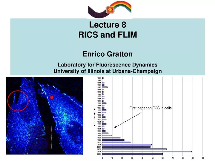
Lecture 8 RICS and FLIM Enrico Gratton Laboratory for Fluorescence Dynamics University of Illinois at Urbana-Champaign. First paper on FCS in cells. INTRODUCTION. Fluctuation Spectroscopy in cells is rapidly expanding Advantages and challenges of FCS in cells

E N D
Lecture 8 RICS and FLIM Enrico Gratton Laboratory for Fluorescence Dynamics University of Illinois at Urbana-Champaign First paper on FCS in cells
INTRODUCTION • Fluctuation Spectroscopy in cells is rapidly expanding • Advantages and challenges of FCS in cells • Single point autocorrelation and cross-correlation provide information on molecular mobility and interactions • PCH provides information on molecular concentration and brightness. Titration experiments in cells • Most studies use fluorescent proteins • Single point FCS is difficult to interpret • Immobile fraction and bleaching perturb the correlation function • Negative-going correlation curves • Different cell locations show different dynamics!
Single point FCS of Adenylate Kinaseb -EGFP Plasma Membrane Cytosol D D Diffusion constants (mm2/s) of AK EGFP-AKb in the cytosol -EGFP in the cell (HeLa). At the membrane, a dual diffusion rate is calculated from FCS data. Away from the plasma membrane, single diffusion constants are found. (Qiaoqiao Ruan, 1999)
time FCS: a closer look at existing techniques Conventional FCS Temporal ICS Time resolution: sec-min Time resolution: μsec-msec Monitors temporal fluctuations at a particular position in the cell to measure relatively faster diffusion (beam transit time in ms). Measurements contain single pixel information. Monitors temporal fluctuations at every point in a stack of 2-D images to measure very slow diffusion (Frame rates in the subsecond range). Measurements contain spatial information (pixel resolution). Can we put the two technologies together?
FCS in cells: Challenges • Need for spatial resolution: Spatio-temporal correlations • Few years ago we proposed scanning FCS (circular orbit) as a method to measure the correlation function at several points in a cell simultaneously (Berland et al, 1995) • N. Petersen and P. Wiseman proposed image correlation spectroscopy (ICS) and recently, time-resolved ICS, similar in concept of scanning FCS in which a point in the image is measured repetitively • These methods have very high spatial resolution but limited time resolution • Scanning correlation in the millisecond • Image correlation in the sub-second • Can we improve the temporal resolution to the level that we can measure freely diffusing molecules, and at the same time have high (pixel) spatial resolution?
FCS: novel ideas • The quick answer is not yet, but we can have a combination of very high time resolution with good spatial resolution. • In addition, there are other major benefits of the technique I will present: • It can be done with commercial laser scanning microscopes (either one or two photon systems) • It can be done with analog detection, as well as with photon counting systems, although the statistics is different • The new technique provides a simple method to account for the immobile fraction • It provides a powerful method to distinguish diffusion from binding • How does it work?
Temporal information hidden in the raster-scan image: the RICS approach Faster diffusion Situation 1:particle is fixed Situation 2: particle is moving Spatial correlation Slower diffusion 1 2 3 4 Pixel (log scale) 1 2 3 4 Situation 1: If the particle is not movingor slowly moving, a signal will be detected at position 1 and 2 but not at 3 and 4. In that case, the correlation between the fluorescence at different pixels will last for the extent of the PSF. Situation 2: If the particle is moving fast, there is a chance to get some signal even at location 3 and 4. The spatial extent of the correlation will increase depending on the time scale of the diffusion. Images obtained in a laser scanning microscope contain temporal information because they are recorded sequentially pixel after pixel as opposed to a camera snap shot. RICS= Raster-scan Image Correlation Spectroscopy
RICS A B Cytosolic Protein Small Molecule Transmembrane Protein Large Protein Aggregates G(t) t=n Line msec Circular/line scan Spatial correlation Circular/line scan Temporal correlation Raster image correlation Frame Temporal correlation Frame sec t=3 t=2 t=1 t=0 Pixel msec 10-6 10-0 10-3 t (s) Available time scales in RICS Range of diffusion times accessible by different RICS techniques. Depending of the time scale of the process, pixel (s), line (ms) or frame (s) correlation methods can be used. Points long a line are microsecond apart. Points in successive lines are millisecond apart and frames are second apart.
time Average Fluorescence t + t t The RICS approach: correlation functions The mathematics and concepts for computation What is different in RICS is the way the correlation function is calculated. We are all familiar with the concept of correlation function of a time series. Definitions: To calculate this function efficiently, the time series must be continuous. Generally, data points are collected every dt. The autocorrelation function is then calculated using either direct numerical algorithms or the FFT method. If the time series is not continuous, but it has regular gaps the correlation function is modulated (convolution with a periodic square wave).
x y The RICS approach: 2-D spatial correlations • In a raster-scan image, points are measured at different positions and at different times simultaneously • If we consider the time sequence, it is not continuous in time • If we consider the “image”, it is contiguous in space • In the RICS approach we calculate the spatial 2-D spatial correlation function (similarly to the ICS method of Petersen and Wiseman) The variables x and y represent spatial increments in the x and y directions, respectively 2-D spatial correlation can be computed very efficiently using FFT methods. To introduce the “RICS concept” we must account for the relationship between time and position of the scanning laser beam.
Effect of diffusion The RICS approach for diffusion We assume that the correlations due to spatial scanning and the correlations due to the dynamics at a point are “independent”: i.e., the dynamics at a point is independent on the scanning motion of the laser beam Consider now the process of diffusion (as one example!). The diffusion kernel can be described by the following expression r Given a particle at the origin at time zero, it can be found at time t at a distance r with a gaussian probability function with standard deviation that increases as a function of time and amplitude that decreases as a function of time
Faster diffusion Spatial correlation Slower diffusion Pixel (log scale) RICS: space and time relationships At any position, the ACF due to diffusion takes the familiar form: tp and tl indicate the pixel time and the line time, respectively. The correlation due to the scanner movement is dr is the pixel size. For D=0 the spatial correlation gives the PSF, with an amplitude equal to 1/N (Petersen and Wiseman). As D increases, the correlation (G term) becomes narrower and the width of the S term increases. Digman et al. Biophys. J., 2005
Performing a RICS measurement • Setup: any laser confocal microscope • Acquire a raster scan image with a pixel time generally in the microsecond range and a line scan time in the millisecond range. • Calculate the 2-D spatial correlation (or RICS analysis). • Fit the 2-D autocorrelation with the previous equations. • For circular or line scanning represent data as pseudo-image, one coordinate being spatial (along the line) and the other being time. This representation allows us to use the RICS approach. The fitting expressions are slightly different (see Digman et al, BJ 2005).
Fit to Correlation Function D = 5.2 ± 0.5 mm2/sec D = 94 ± 9mm2/sec RICS: Fit of spatial correlation functions Simulations Spatial correlation function Image 10 nm beads EGFP in a plane 256x256, 16 s/pixel, 0.050 m/pixel Digman et al. Biophys. J., 2005.
RICS: Fits to spatial correlation functions Olympus Fluoview300 LSM EGFP in solution Spatial ACF 128x128, 4 s/pixel, 5.4 ms/line, 0.023 m/pixel Fit to Spatial ACF D = 105 ± 10m2/s Digman et al. Biophys. J., 2005
Testing RICS For molecules in solution, the method works fine. The same G(0) and the same D is obtained using single point FCS or the RICS calculation. Simulations: comparison between 3 different methods to recover D and G(0) for 2 different values of D (100 mm2/s and 6 mm2/s). Conditions: Sampling frequency was 128 kHz for the fast moving particle and 32 kHz for the slowly diffusing particle. The orbit was sample at 128 points and the frame for the raster scan was 128x128 pixels. 1.6M points were simulated in each run irrespective of the sample frequency. Experimental data: fluorescent bead diffusing in solution
RICS benefits: better S/N at low concentrations Repetition of 10 runs Repetitions of the same simulation (N=10) to estimate standard deviations. 100 particle diffusing in a plane of 128x128 pixels of 0.05m each detected by different methods and recovered by the different equations. The length of the data stream is the same for each simulation, 320k points were simulated.
How we go from solutions to cells? In cells we have an immobile fraction: molecules not moving during the course of the experiment. If we perform the 2-D-image correlation operation of an image that contains immobile features, we obtain the transform (power spectrum) of the image. In this transform is impossible to distinguish the moving particles. We need to separate this immobile fraction from the mobile part before calculating the transform How is this achieved?
Photon counting: ACF of a bright immobile particle t Analog detection: ACF of a bright immobile particle t RICS: subtraction of immobile features Basic idea In a “truly immobile” bright region, at each pixel the intensityfluctuates according to the Poisson distribution. However the time correlation of the shot noise is zero, except at channel zero. Also, if we cross-correlate the intensity at any two pixels, even if very close (within the PSF), the cross-correlation due to shot noise is zero. Therefore, if we subtract the average intensity and disregard the zero time-space point, the immobile bright region totally disappear from the correlation function (in the first approximation). After subtraction of the average image, a small number (equal to the image intensity is added). Attention!!!! This is not true for analog detection, not even in the first order approximation. For analog detection the shot noise is time (and space) correlated.
detail RICS -average Subtraction of the immobile fraction The stack of images contains both mobile and immobile bright particles. The correlation function mostly reflects the shape of the immobile bright particles. After subtraction, the RICS only shows the fast diffusing molecules! original image RICS The stack of images contains only mobile particles. The RICS and the subtracted RICS are identical RICS original image The same method can be used to subtract very slowly moving structure to account for the cell movement
RICS: Immobile Component Removal Paxillin-EGFP in CHO K1 Region of Interest ACF with Immobile ACF no Immobile 64x64, 8 s/pixel, 5.4 ms/line, 0.023 m/pixel Fit to ACF with Immobile Component Removed D = 0.49 ± 0.05m2/s Digman et al. Biophys. J., 2005
Photon counting: ACF of a bright immobile particle t RICS: Removal of slowly varying component Very often cells (or parts of the cell) move. Instead of subtracting the average (over the entire image stack), we could subtract a local moving average. This is equivalent to high-pas filtering of the image: only the fast changing features remain. In our software, it is possible to use different moving average lengths, depending on the speed of motion of the quasi immobile features. Warning: The principle that the shot noise is time and space uncorrelated is not valid. After high-pass filtering, the intensity of one pixel carries to the next, both in time and in space, introducing correlations that were not there originally. However, the effect of filtering can be predicted and recognized. High pass filter effect: ACF of a bright slowly mobile particle t Effect of HPF
(with moving average of 10) Example: GAP-GFP Small peptide that anchors GFP to the membrane 2-D spatial correlation Average image of a 64x64 ROI Original image (128x128) 700 frames Recovered diffusion parameters for the mobile fraction G(0) = 0.020 D = 0.50 μm2/s Note that the diffusion coefficient recovered is an average over the entire ROI analyzed: the spatial resolution is dependent on the size of the ROI. Fit of the 2-D spatial correlation
RICS: Spatio-temporal correlations Diffusion or binding? (or blinking) • Frequently, we obtain apparent diffusion coefficients below 0.01 mm2/s. These values are highly suspicious for single molecules or small aggregates! • Experimentally it is difficult to distinguish between binding (exponential functions) and diffusion. PCH analysis often show that the amplitude fluctuations correspond to few fluorescent molecules. • The original work of Elson, Magde and Webb in FCS was to measure binding. • In solution is possible to predict the value of the diffusion; in cell this is problematic. • The spatial correlation resulting from binding to immobile structures is different from diffusion. • RICS could identify binding (to immobile structures), blinking of diffusing particles and pure diffusion.
RICS: Models Diffusion or binding? (or blinking) For pure “binding equilibria” the function G(x,y) assumes a different expression Line scan measurement (Fluoview300). Fit (black line) of pixel 190 data (red line) of the line scan experiment using A) diffusion equation D=0.032mm2/s and B) using exponential relaxation t=0.63 s. The residues (blue lines) of the exponential fit are smaller and less correlated indicating a better fit using the exponential model
Binding site RICS: Models Diffusion or binding? (or blinking) Slowly diffusing Diffusion is faster than binding The RICS correlation function should be identical to the PSF. The amplitude should correspond to the brightness of the particle binding. Adjacent points should be uncorrelated. The binding kinetics is independent on the beam waist. If there is only one binding site (or few), we could obtain directly the on-off statistics. Diffusion is very slow The RICS correlation function should be slightly broadened. The amplitude should correspond to the brightness of the particle. Adjacent points could be correlated. The diffusion kinetics depends on the square of the beam waist
RICS: Models Unimolecular reaction K = kf / kbis the equilibrium coefficient; l = kf + kb is the apparent reaction rate coefficient; and fj is the fractional intensity contribution of species j Note that diffusion modifies the shape of the spatial correlation function while binding equilibria gives always the same shape (the PSF) assuming that diffusion is fast compared to binding rate (either the on or the off rate)
RICS: Summary of spatial and time resolution Resolution of the various scan methods Digman et al. Biophys. J., 2005
RICS: Conclusions • There is a hidden time structure in the laser scanning images that can be exploited to obtain information about • Diffusion • Velocity • Brightness • Aggregation • Blinking, binding-unbinding equilibria • We developed a general method to separate mobile from immobile fraction • This new development has great potential consequences for anyone interested in cellular imaging and dynamics
Globals by Enrico Gratton Gs Gi spectroscopy images The Globals program originally developed at the LFD for analysis of multiple files from spectroscopy is now available for image analysis. This new program analyzes FCS in images by the RICS approach, and lifetime images using the phasor approach. Available in the Fall of 2005. Price $1000 for Globals for Spectroscopy $1000 for Globals for Images More information at www.lfd.uiuc.edu
GLOBALS for IMAGES derives from SimFCS • It is intended for analysis of images using physical models • Has the same minimization engine and error analysis of the original Globals Unlimited program • It has a very extensive library for analysis of • FCS • RICS • FLIM • SPT • 2-D and 3-D representations of data • Reads most of the file formats (B&H, FIFO, TIF, Methamorph, LSM, binary) • The emphasis is on model analysis (not image processing)
Ultrafast Analysis of Fluorescence Lifetime Images using the Phasor approach: Application to FRET analysis Enrico Gratton University of California at Irvine
Introduction FLIM (fluorescence lifetime imaging microscopy) is becoming an important technique in fluorescence imaging microscopy. FLIM is used for FRET Ion concentration In a FLIM experiment, the fluorescence lifetime is measured at every single point in a image, generally 256x256 pixels There are technical challenges regarding how to achieve the necessary data acquisition speed A major problem is data analysis and interpretation
The challenges of FLIM At every pixel there are contributions of several fluorescent species, each one could be multi-exponential. To make things worse, we can only collect light for a limited amount of time (100-200 microseconds per pixel) which result in about 500-1000 photons per pixel. This is barely enough to distinguish a double exponential from a single exponential decay. Resolving the decay at each pixel in multiple components is a complex computational task “for experts only”, partially alleviated by extensive use of global techniques.
Major issues with FLIM • Rather difficult technique • Long times for calculations • Results depend on initial conditions • Interpretation requires expertise • Can we avoid all these problems? • No expertise necessary • Instantaneous results • Independent on initial choices • Quantitative results • Intuitive simple interface
A new approach • Presently, the analysis proceed by resolving the exponential components at each pixel and by identifying molecular species with lifetime components. • In the microscope environment, this process is prone to errors and depends on interpretation. • We propose a change in paradigm: Use a different representation of the decay where each molecular species has its own unique representation and where each process (FRET, ion concentration changes) is easily identified. • We need to go to a new “space”.
The phasor space and the universal circle (From Star-Trek) • When a fluorescent sample is excited with a sinusoidally modulated light, it responds with emission that has the same frequency but is phase shifted and demodulated with respect to excitation. • Where does this concept come from?? • We need some math. This is what we need: the phaser! Where does this concept come from?
M phase What is a phasor?? • A phasor is a quantity like a vector. Phasors can be added like vectors. You need to calculate the vector components and then add the components to obtain the vector sum s g
How to calculate the components g and s of a phasor from the time decay? Frequency-domain components of a phasor. m and f is what is measured Time-domain components of a phasor. I(t) is what is measured Note that I(t) is not resolved in components!!
DC n1 n1 n2 n3 n4 DC:=(n1+n2+n3+n4)/4 AC2=(n1-n3)2+(n2-n4)2 f=tan-1(n2-n4)/(n1-n3) M=AC/DC One period Calculation of phase and modulation: frequency domain
Calculation of phase and modulation: time domain n1 n2 n3 n4 n1 DC:=(n1+n2+n3+n4)/4 AC2=(n1-n3)2+(n2-n4)2 f=tan-1(n2-n4)/(n1-n3) M=AC/DC One period We use identical formulas!!!
The algebra of phasors A Phasor B Phase delay emission m s Φ g 1 excitation C t2 t2 min Experimental point t1 max f1 t1 f2 1 1 Universal circle Lifetime representation using phasors. A: Rotating vectors for excitation an demission with different phase delay. B: As the modulation frequency increases the end of the phasor describes a semicircle of radius ½ and centered at (½, 0). C) Mixtures of t1 and t2 must be on the line between t1 and t2 in proportion to their fractional intensity contribution. Given the experimental point and t1 we can find t2 and the fractional contribution. Given the experimental point, t1 must be less than t1 max and t2 must be greater than a t2 min.
Quenching trajectory Experimental point P2 P2 P1 f2 P1 1 1 B A How to distinguish two-exponential components from FRET? Exponential components fall on the semicircle. A) Decay components made of multi-exponentials can fall any where. A linear combination of the two decays must fall in the line between the two decays. B) If there is quenching of t2 (the donor) the experimental values of experimental phasor cannot be on the line joining t2 to t1. Quenching trajectories can be very curved since t2 could become smaller that t1 depending on the FRET efficiency.
2000 c b d a 0 Example of FLIM analysis using phasors Several regions the image can be identified corresponding to a) background (2 exponentials b) cell 1 bright (2 exponentials) c) cell 2 dim, d) cell junctions dim. Image of cell expressing uPAR-EGFP and uPAR-MRFP receptor. Upon addition of a ligand, the receptor aggregates. FRET should occur at the cell junctions
2000 5 ns C A B 0 0 ns ns ns The pitfall of “conventional” FLIM analysis Image obtained using B&H 830 in our 2-photon microscope Shorter lifetime region could be interpreted to be due to FRET Donor+acceptor+ligand. A) intensity image after background subtraction, B) tp image C) tm image.
2000 C D B C A 0 B’ A’ C’ Identification of FRET using the phasor plot FRET only occurs at the cell junctions Selecting regions of the phasor diagram. Selecting the region in A’ (donor +acceptor) the part in white lights up (A). Selecting the region in B’ (autofluorescence) the part in white in lights up (B). The color scale in B’ has been changed to better show the region of the autofluorescence. Selecting the region in C’ (along the donor quenching line as shown in D) the part in white in at the cell junction lights up in C.
How to identify components? Phasors for common fluorophores. EGFP (green), CFP (blue) mRFP1 (red), autofluorescence (at 880 nm -2photon excitation) violet. In any given pixel, mixture of EGFP and autofluorescence must be on the yellow line, mixtures of EGFP and mRFP1 must be on the red line. Mixtures of three of them must be inside the triangle with the corner in the 3 phasors.
How to identify processes? Delay Quenching Donor Acceptor Delay of the excitation of the acceptor due to FRET moves the acceptor phasor to the left (yellow arrow). If the delay is sufficiently long, the phasor could fall outside the semicircle. The donor phasor moves to the right (red arrow) due to quenching (shorter lifetime).
Features of the new approach Many of the obstacles in FLIM data analysis can be removed. The accuracy of lifetime determination improved. The speed of data analysis reduced to be almost instantaneous for an entire image and also using several (>10) images simultaneously. The analysis is “global” over the image and across images. The interpretation of the FLIM experiment is straightforward. Minimal prior spectroscopy knowledge needed. The tool can be applied to all modes of data acquisition (frequency-domain and time-domain)
Raichu FLIM/FRET analysis In MEF cells http://www.biken.osaka-u.ac.jp/biken/shuyouvirus/e-phogemon/raichu-Rac.htm