Download

1 / 59
590 likes | 881 Views
Face Recognition in Subspaces. 601 Biometric Technologies Course. Abstract. Images of faces, represented as high-dimensional pixel arrays, belong to a manifold (distribution) of a low dimension.

E N D
Face Recognition in Subspaces 601 Biometric Technologies Course
Abstract • Images of faces, represented as high-dimensional pixel arrays, belong to a manifold (distribution) of a low dimension. • This lecture describes techniques that identify, parameterize, and analyze linear and non-linear subspaces, from the original Eigenfaces technique to the recently introduced Bayesian method for probabilistic similarity analysis. • We will also discuss comparative experimental evaluation of some of these techniques as well as practical issues related to the application of subspace methods for varying pose, illumination, and expression.
Outline • Face space and its dimensionality • Linear subspaces • Nonlinear subspaces • Empirical comparison of subspace methods
Face space and its dimensionality • Computer analysis of face images deals with a visual signal that is registered by a digital sensor as an array of pixel values. The pixels may encode color or only intensity. After proper normalization and resizing to a fixed m-by-n size, the pixel array can be represented as a point (i.e. vector) in a mn-dimensional image space by simply writing its pixel values in a fixed (typically raster) order. • A critical issue in the analysis of such multidimensional data is the dimensionality, the number of coordinates necessary to specify a data point. Bellow we discuss the factors affecting this number in the case of face images.
Image space versus face space • Handling high-dimensional examples, especially in the context of similarity and matching based recognition, is computationally expensive. • For parametric methods, the number of parameters one needs to estimate typically grows exponentially with the dimensionality. Often, this number is much higher than the number of images available for training, making the estimation task in the image space ill-posed. • Similarly, for nonparametric methods, the sample complexity - the number of examples needed to represent the underlying distribution of data efficiently – is prohibitively high.
Image space versus face space • However, much of the surface of a face is smooth and has regular texture. Per pixel sampling is in fact unnecessarily dense: the value of a pixel is highly correlated to the values of surrounding pixels. • The appearance of faces is highly constrained: i.e., any frontal view of a face is roughly symmetrical, has eyes on the sides, nose in the middle etc. A vast portion of the points in the image space does not represent physically possible faces. Thus, the natural constraints dictate that the face images are in fact confined to a subspace referred to as the face space.
Principal manifold and basis functions • Consider a straight line in R3, passing through the origin and parallel to the vector a=[a1, a2 ,a3]T . • Any point on the line can be described by 3 coordinates; the subspace that consists of all points on the line has a single degree of freedom, with the principal mode corresponding to translation along the direction of a. Representing points in this subspace requires a single basis function: • The analogy here is between the line and the face space and between R3 and the image space.
Principal manifold and basis functions • In theory, according to the described model any face model should fall in the face space. In practice, owing to sensor noise, the signal usually has a nonzero component outside of the face space. This introduces uncertainty into the model and requires algebraic and statistical techniques capable of extracting the basis functions of the principal manifold in the presence of noise.
Principal component analysis • Principal component analysis (PCA) is a dimensionality reduction technique based on extracting the desired number of principal components of the multidimensional data. • The first principal component is the linear combination of the original dimensions that has maximum variance. • The n-th principal component is the linear combination with the highest variance subject to being orthogonal to the n-1 first principal components.
Principal component analysis • The axis labeled Φ1 corresponds to the direction of the maximum variance and is chosen as the first principal component. In a 2D case the 2nd principal component is then determined by the orthogonality constraints; in a higher-dimensional space the selection process would continue, guided by the variance of the projections.
Principal component analysis • PCA is closely related to the Karhunen-Loève Transform (KLT) which was derived in the signal processing context as the orthogonal transform with the basis Φ = [Φ1,…, ΦN]T that for any k<=N minimizes the average L reconstruction error for data points x. • One can show that under the assumption that the data are zero-mean, the formulations of PCA and KLT are identical, without loss of generality, we assume that the data are indeed zero-mean; that is the mean face x is always subtracted from the data.
Principal component analysis • Thus, to perform PCA and extract k principal components of the data, one must project the data onto Φk, the first k columns of the KLT basis Φ, which correspond to the k highest eigenvalues of Σ. This can be seen as a linear projection RN--> Rk, which retains the maximum energy (i.e. variance) of the signal. • Another important property of PCA is that it decorrelates the data: the covariance matrix of ΦkT X is always diagonal.
Principal component analysis • PCA may be implemented via singular value decomposition (SVD). The SVD of a MxN matrix X (M>=N) is given by X=U D V T, where the MxN matrix U and the NxN matrix V have orthogonal columns, and the NxN matrix D has the singular values of X on its main diagonal and zero elsewhere. • It can be shown that U = Φ, so SVD allows sufficient and robust computation of PCA without the need to estimate the data covariance matrix Σ. When the number of examples M is much smaller than the dimension N, this is a crucial advantage.
Eigenspectrum and dimensionality • An important largely unsolved problem in dimensionality reduction is the choice of k, the intrinsic dimensionality of the principal manifold. No analytical derivation of this number for a complex natural visual signal is available to date. To simplify this problem, it is common to assume that in the noisy embedding of the signal of interest (a point sampled from the face space) in a high dimensional space, the signal-to-noise ratio is high. Statistically. That means that the variance of the data along the principal modes of the manifold is high compared to the variance within the complementary space. • This assumption related to the eigenspectrum, the set of eigenvalues of the data covariance matrix Σ. Recall that the i-th eigenvalue is equal to the variance along the i-th principal component. A reasonable algorithm for detecting k is to search for the location along the decreasing eigenspectrum where the value of λi drops significantly.
Outline • Face space and its dimensionality • Linear subspaces • Nonlinear subspaces • Empirical comparison of subspace methods
Linear subspaces • Eigenfaces and related techniques • Probabilistic eigenspaces • Linear discriminants: Fisherfaces • Bayesian methods • Independent component analysis and source separation • Multilinear SVD: “Tensorfaces”
Linear subspaces • The simplest case of principal manifold analysis arises under the assumption that the principal manifold is linear. After the origin has been translated to the mean face (the average image in the database) by subtracting it from every image, the face space is a linear subspace of the image space. • Next we describe methods that operate under the assumption and its generalization, a multilinear manifold.
Eigenfaces and related techniques • In 1990, Kirby and Sirovich proposed the use of PCA for face analysis and representation. Their paper was followed by the eigenfaces technique by Turk and Pentland, the first application of PC to face recognition. The basis vectors constructed by PCA had the same dimension as the input face images, they were named eigenfaces. • Figure 2 shows an example of the mean face and a few of the top eigenfaces. Each face image was projected into the principal subspace; the coefficients of the PCA expansion were averaged for each subject, resulting in a single k-dimensional representation of that subject. • When a test image was projected into the subspace, Euclidian distances between its coefficient vector and those representing each subject were computed. Depending on the distance to the subject for which this distance would be minimized and the PCA reconstruction error, the image was classified as belonging to one of the familiar subjects, as a new face or as a nonface.
Probabilistic eigenspaces • The role of PA in the original Eigenfaces was largely confined to dimensionality reduction. The similarity between images I1 and I2 was measured in terms of the Euclidian norm of the difference Δ = I1- I2 projected to the subspace, essentially ignoring the variation modes within the subspace and outside it. This was improved in the extension of eigenfaces proposed by Moghaddam and Pentland, which uses a probabilistic similarity measure based on a parametric estimate pf the probability density p(Δ|Ω). • A major difficulty with such estimation is that normally there are not nearly enough data to estimate the parameters of the density in a high dimensional space.
Linear discriminants: Fisherfaces • When substantial changes in illumination and expression are present, much of the variation in the data is due to these changes. The PCA techniques essentially select a subspace that retains most of that variation, and consequently the similarity in the face space is not necessarily determined by the identity.
Linear discriminants: Fisherfaces • Belhumeur et al. propose to solve this problem with Fisherfaces, an application of Fisher;s linear discriminant FLD. FLD selects the linear subspace Φ which maximizes the ratio • is the within-class scatter matrix; m is the number of subjects (classes) in the database. FLD finds the projection of data in which the classes are most linearly separable.
Linear discriminants: Fisherfaces • Because in practice Sw is usually singular, the Fisherfaces algorithm first reduces the dimensionality of the data with PCA and then applies FLD to further reduce the dimensionality to m-1. • The recognition is then accomplished by a NN classifier in this final subspace. The experiments reported by Belhumeur et al. were performed on data sets containing frontal face images of 5 people with drastic lighting variations and another set with faces of 16 people with varying expressions and again drastic illumination changes. In all the reported experiments Fisherfaces achieve a lower rate than eigenfaces.
Bayesian methods • By PCA, the Gaussians are known to occupy only a subspace of the image space (face space); thus only the top few eigenvectors of the Gaussian densities are relevant for modeling. These densities are used to evaluate the similarity. Computing the similarity involves subtracting a candidate image I from a database example Ij. • The resulting Δ image is then projected onto the eigenvectors of the extrapersonal Gaussian and also the eigenvectors of the intrapersonal Gaussian. The exponential are computed, normalized, and then combined. This operation is iterated over all examples in the database, and the example that achieves the maximum score is considered the match. For large databases, such evaluations are expensive and it is desirable to simplify them by off-line transformations.
Bayesian methods • After this preprocessing, evaluating the Gaussian can be reduced to simple Euclidean distances. Euclidean distances are computed between the kI-dimensional yΦI as well as the kE-dimensional yΦE vectors. Thus, roughly 2x(kI+ kE) arithmetic operations are required for each similarity computation, avoiding repeated image differencing and projections. • The maximum likelihood (ML) similarity is even simpler, as only the intrapersonal class is evaluated, leading to the following modified form for similarity measure. • The approach described above requires 2 projections of the difference vector Δ from which likelihoods can be estimated for the bayesian similarity measure. The projection steps are linear while the posterior computation is nonlinear.
Bayesian methods • Fig. 5.ICA vs PCA decomposition of a 3D data set. • The bases of PCA (orthogonal) and ICA (non-orthogonal) • Left: the projection data onto the top 2 principal components (PCA). Right: the projection onto the top two independent components (ICA)
Independent component analysis and source separation • While PCA minimizes the sample covariance (second-order dependence) of data, independent component analysis (ICA) minimizes higher-order dependencies as well, and the components found by ICA are designed to be non-Gaussian. Like PCA, ICA yields a linear projection but with different properties: x~Ay, AT A ≠I, P(y) ~ Π p(yi) • That is, approximate reconstruction, nonorthogonality of the basis A, and the near-factorization of the joint distribution P(y) into marginal distributions of the (non-Gaussian) ICs.
Independent component analysis and source separation • Basis images obtained with ICA: Architecture I (top), and II (bottom).
Multilinear SVD: “Tensorfaces” • The linear analysis methods discussed above have been shown to be suitable when pose, illumination, or expression are fixed across the face database. When any of these parameters is allowed to vary, the linear subspace representation does not capture this variation well. • In the following section we discuss recognition with nonlinear subspaces. An alternative, multilinear approach, called tesorfaces has been proposed by Vasilescu and Terzopolous.
Multilinear SVD: “Tensorfaces” • Tensor is a multidimensional generalization of a matrix: an n-order tensor A is an object with n indices, with elements denoted by ai1, …,inЄ R. Note that there are n ways to flatten this tensor (e.g. to rearrange the elements in a matrix): The i-th row of A(s) is obtained by concatenating all the elements of A of the form ai1, …,is-1, i, is+1,…,in.
Multilinear SVD: “Tensorfaces” • Fig. Tensorfaces • Data tensor; the 4 dimensions visualized are identity, illumination, pose, and the pixel vector; the 5th dimension corresponds to expression (only the subtensor for neutral expression is shown) • Tensorfaces decomposition.
Multilinear SVD: “Tensorfaces” • Given an input image x, a candidate coefficient vector cv,i,e is computed for all combinations of viewpoint, expression, and illumination. The recognition is carried out by finding the value of j that yields the minimum Euclidean distance between c and the vectors cj across all illuminations, expressions and viewpoints. • Vasilescu and Terzopolous reported experiments involving the data tensor consisting of images of Np = 28 subjects photographed in Ni = 3 illumination conditions from Nv=5 viewpoints with Ne=3 different expressions. The images were resized and cropped so they contain N=7493 pixels. The performance of tensorfaces is reported to be significant better than that of standard eigenfaces.
Outline • Face space and its dimensionality • Linear subspaces • Nonlinear subspaces • Empirical comparison of subspace methods
Nonlinear subspaces • Principal curves and nonlinear PCA • Kernel-PCA and Kernel-Fisher methods Fig. (a) PCA basis (linear, ordered and orthogonal) (b) ICA basis (linear, unordered, and nonorthogonal) (c) Principal curve (parameterized nonlinear manifold). The circle shows the data mean.
Principal curves and nonlinear PCA • The defining property of nonlinear principal manifolds is that the inverse image of the manifold in the original space RN is a nonlinear (curved) lower-dimensional surface that “passes through the middle of data’ while minimizing the sum total distance between the data point and their projections on that surface. Often referred as principal curves this formulation is essentially a nonlinear regression on the data. • One of the simplest methods for computing nonlinear principal manifolds is the nonlinear PCA (NLPCA) autoencoder multilayer neural network The bottleneck layer forms a lower dimensional manifold representation by means of a nonlinear projection function f(x), implemented as a weighted sum-of-sigmoids. The resulting principal components y have an inverse mapping with similar nonlinear reconstruction function g(y) which reproduces the input data as accurately as possible. The NLPCA computed by such a multilayer sigmoidal neural network is equivalent to a principal surface under the more general definition.
Principal curves and nonlinear PCA • Fig 9. Autoassociative (“bottleneck”) neural network for computing principal manifolds
Kernel-PCA and Kernel-Fisher methods • Recently nonlinear principal component analysis was revived with the “kernel eigenvalue” method of Scholkopf et al. The basic methodology of KPCA is to apply a nonlinear mapping to the input Ψ(x):RNRL and then to solve for linear PCA in the resulting feature space RL,where L is larger than N and possibly infinite. Because of this increase in dimensionality, the mapping Ψ(x) is made implicit (and economical) by the use of kernel functions satisfying Mercer’s theorem • k(xi, xj) = [Ψ(xi) * Ψ(xj) ] • Where kernel evaluations k(xi, xj) in the input space correspond to dot-products in the higher dimensional feature space.
Kernel-PCA and Kernel-Fisher methods • A significant advantage of KPCA over neural network and principal cures is that KPCA does not require nonlinear optimization, is not subject of overfitting, and does not require knowledge of the network architecture or the number of dimensions. Unlike traditional PCA, one can use more eigenvector projections than the input dimensionality of the data because KPCA is based on the matrix K, the number of eigenvectors or features available is T. • On the other hand, the selection of the optimal kernel remains an “engineering problem” . Typical kernels include Gaussians exp(-|| xi- xj ||)2/δ2), polynomials (xi* xj)d and sigmoids tanh (a(xi* xj)+b), all which satisfy Mercer’s theorem.
Kernel-PCA and Kernel-Fisher methods • Similar to the derivation of KPCA, one may extend the Fisherfaces method by applying the FLD in the feature space. Yang derived the kernel space through the use of the kernel matrix K. In experimenst on 2 data sets that contained images from 40 and 11 subjects, respectively, with varying pose, scale, and illumination, this algorithm showed performance clearly superior to that of ICA, PCA, and KPCA and somewhat better than that of the standard Fisherfaces.
Outline • Face space and its dimensionality • Linear subspaces • Nonlinear subspaces • Empirical comparison of subspace methods
Empirical comparison of subspace methods • Moghaddam reported on an extensive evaluation of many of the subspace methods described above on a large subset of the FERET data set. The experimental data consisted of a training “gallery” of 706 individual FERET faces and 1123 “probe” images containing one or more views of every person in the gallery. All these images were aligned reflected various expressions, lighting, glasses on/off, and so on. • The study compared the Bayesian approach to a number of other techniques and tested the limits of recognition algorithms with respect to a image resolution or equivalently the amount of visible facial detail.
Empirical comparison of subspace methods • Fig 10. Experiments on FERET data. (a) Several faces from the gallery. (b) Multiple probes for one individual, with different facial expressions, eyeglasses, variable ambient lighting, and image contrast. (c) Eigenfaces. (d) ICA basis images.
Empirical comparison of subspace methods • The resulting experimental trials were pooled to compute the mean and standard derivation of the recognition rates for each method. The fact that the training and testing sets had no overlap in terms of individual identities led to an evaluation of the algorithm’s generalization performance – the ability to recognize new individuals who were not part of the manifold computation or density modeling with the training set. • The baseline recognition experiments used a default manifold dimensionality of k=20.
PCA-based recognition • The baseline algorithm for these face recognition experiments was standard PCA (eigenface) matching. • Projection of the test set probes onto the 20-dimensional linear manifold (computed with PCA on the training set only) followed by the nearest-neighbor matching to the approx. 140 gallery images using Euclidean metric yielded a recognition rate of 86.46%. • Performance was degraded by the 252 20 dimensionality reduction as expected.
ICA-based recognition • 2 algorithms were tried : the “JADE” algorithm of Cardoso and the fixed-point algorithm of Hyvarien and Oja, both using a whitening step (“sphering”) preceding the core ICA decomposition. • Little difference between the 2 ICA algorithms was noticed and ICA resulted in the latest performance variation in the 5 trials (7.66% SD). • Based on the mean recognition rates it is unclear whether ICA provides a systematic advantage over PCA or whether “more non-Gaussian” and/or “more independent” components result in a better manifold for recognition purposes with this dataset.
ICA-based recognition • Note that the experimental results of Barlett et al. with FERET faces did favor ICA over PCA. This seeming disagreement can be reconciled if one considers the differences in the experimental setup and the choice of the similarity measure. • First, the advantage of ICA was seen primarily with more difficult time-separated images. In addition, compared to the results of Barlett et al. the faces in this experiment were cropped much tighter, leaving no information regarding hair and face shape, an they were much lower resolution, factors that combined make the recognition task much more difficult. • The second factor is the choice of the distance function used to measure similarity in the subspace. This matter was further investigated by Draper et al. they found that the best results for ICA are obtained using the cosine distance, whereas for eigenfaces the L1 metric appears to be optimal; with L2 metric, which was also used in the experiments of Moghaddam, the performance of ICA was similar to that of eigenfaces.