Download
1 / 14
140 likes | 306 Views
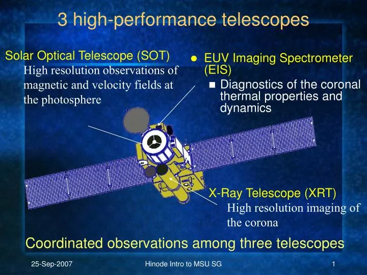
EUV Imaging Spectrometer (EIS) Diagnostics of the coronal thermal properties and dynamics. 3 high-performance telescopes. Solar Optical Telescope (SOT) High resolution observations of magnetic and velocity fields at the photosphere. X-Ray Telescope (XRT) High resolution imaging of the corona.

E N D
EUV Imaging Spectrometer (EIS) Diagnostics of the coronal thermal properties and dynamics 3 high-performance telescopes • Solar Optical Telescope (SOT) • High resolution observations of magnetic and velocity fields at the photosphere • X-Ray Telescope (XRT) • High resolution imaging of the corona Coordinated observations among three telescopes Hinode Intro to MSU SG
Hinode Fields of View 800arcsec 360arcsec 320arcsec 512arcsec 160arcsec SOT EIS 2000arcsec XRT Maximum size of FOV is shown here. Hinode Intro to MSU SG
Optical Path X-Ray Mirror Shutter & filter wheels Visible Light Optic Focus Mechanism Hinode Intro to MSU SG
Focal Plane Filter Wheels Hinode Intro to MSU SG
Observational Constraints • Three basic types of XRT observations, which must be optimized subject to our data rate (~ 0.5 Gbyte/day) • Thermal structure & energetics • 3-7 filters used per target region • May limit cadence or FOV to stay within the data rate. • Dynamics • Fast cadence with 1 or 2 filters • May limit context images or FOV to stay within the data rate • Morphology / Topology • Large FOV, combine long and short exposures • May limit number of filters, cadence or FOV Hinode Intro to MSU SG
What kind of images will you find? • Full-Sun synoptic images, 2-4 times per day, several filters • Partial-Sun images, throughout the day • Field of view 384x384, 512x512, and some 1024x384 • Active regions, coronal holes, quiet sun, variety of targets • Sometimes a single filter at high cadence • Sometimes many filters for temperatures, DEMs • And with occasional full-Sun images for context Hinode Intro to MSU SG
What format? What level of preparation? • FITS format, with time/date/filter/pointing info in the header • Level-0 data have complete header info, but no preparation • No corrections for dark current, exposure time, jitter: They’re Raw. • Preparation software are available in SolarSoft • Typically available a few days after the image was made. Hinode Intro to MSU SG
Finding the Data: VSO • VSO • http://sdac.virtualsolar.org/cgi-bin/search • Check ‘Instrument/Source/Provider’ and select ‘Generate VSO Search Form’ • Select date & time interval • Check ‘SAO’ (for now) and ‘XRT’ and hit ‘Search’ • Use the checkboxes to choose the data you want • The “All above” or “All below” options may be useful. Hinode Intro to MSU SG
Finding the Data: SOT website • SOT website at LMSAL • http://sot.lmsal.com/sot-data • Choose ‘Planned’ for a link to what’s planned in the next day or so. Descriptive, but the data aren’t there. • Choose ‘Recent’ for a link to recently acquired data. • Select ‘XRT’ • Click on an image for a link to more data from that set. • These are automatically generated, so the results of this method are hard to predict. I haven’t had much luck with them, but I’m impatient. Hinode Intro to MSU SG
Finding the Data: xrt_cat • xrt_cat in SolarSoft • Take advantage of MSU’s data archive • On jefferson: IDL> t0 = '2007-03-26T17:00:00' IDL> t1 = '2007-03-26T18:10:00' IDL> xrt_cat, t0, t1, catx, ofiles IDL> help, catx CATX STRUCT = -> <Anonymous> Array[126] IDL> help, ofiles OFILES STRING = Array[126] IDL> print, ofiles(0:1) /disk/data/HINODE/xrt/level0/2007/03/26//H1700/XRT20070326_170036.9.fits /disk/data/HINODE/xrt/level0/2007/03/26//H1700/XRT20070326_170050.1.fits Hinode Intro to MSU SG
Reading the Data on jefferson • Two choices IDL> mreadfits, ofiles, index, data IDL> read_xrt, ofiles, index, data, /force • Example of selecting only images of a certain size IDL> ss = where(catx.naxis1 eq 512 and catx.naxis2 eq 512) IDL> read_xrt, ofiles(ss), index, data Hinode Intro to MSU SG
Prepping the Data on jefferson • An example IDL> ss = where(catx.naxis1 eq 512 and catx.naxis2 eq 512) IDL> read_xrt, ofiles(ss), index, data IDL> xrt_prep, index, data index_out, data_out, /norm, /float [or] IDL> xrt_prep, ofiles, ss, index_out, data_out, /norm, /float Hinode Intro to MSU SG
Advanced Topics • Removing spacecraft jitter IDL> xrt_prep, index_in, data_in, index_prep, data_prep, /norm, /float IDL> ssw_path, '/ssw/hinode/xrt/idl/util/jitter' IDL> xrt_jitter, index_prep, jitter_offset IDL> data_out = image_translate(data_prep, jitter_offset, /interp) • Removing CCD contamination spots Hinode Intro to MSU SG
End Presentation Hinode Intro to MSU SG