Download

1 / 45
450 likes | 456 Views
Should we forget the Smith Predictor?. Chriss Grimholt Sigurd Skogestad Department of Chemical Engineering, NTNU, Trondheim, Norway. IFAC PID’18. TexPoint fonts used in EMF. Read the TexPoint manual before you delete this box.: A A A A A A A A A. Outline. What is a good controller?

E N D
Should we forget the Smith Predictor? Chriss Grimholt Sigurd Skogestad Department of Chemical Engineering, NTNU, Trondheim, Norway IFAC PID’18 TexPoint fonts used in EMF. Read the TexPoint manual before you delete this box.: AAAAAAAAA
Outline • What is a good controller? • Performance, IAE • Robustness, Ms • Delay margin • Smith Predictor (Time delay compensator) • Optimal Smith-Predictor vs. Optimal PI/PI for first-order plus delay plants • Trade-off plots (IAE vs. Ms) • Delay margin • Simulations • Why is Smith Predictor not robust? • Comparison with SIMC PI tuning rules • Conclusion
1. What is a good controller? High controller gain (“tight control”) Low controller gain (“smooth control”) • Multiobjective. Tradeoff between • Output performance • Robustness • Input usage • Noise sensitivity Our choice: • Quantification • Output performance: • Frequency domain: weighted sensitivity ||WpS|| • Time domain: IAE or ISE for setpoint/disturbance • Robustness: Ms, Mt, GM, PM, Delay margin, … • Input usage: ||KSGd||, TV(u) for step response • Noise sensitivity: ||KS||, etc. J = avg. IAE for Setpoint & disturbance Ms = peak sensitivity IAE=Integrated absolute error
Output performance (J): Integrated absolute error (IAE) IAE = Integrated absolute error = ∫|y-ys|dt, for step change in ys or d
Delay margin DM = «How much extra time delay we can add to the loop before the system goes unstable» Not guaranteed by MST
2. Smith Predictor (SP) c Our case G0 = k/(τs+1) K = Kc(1+1/τIs)(PI controller). Internal model control (IMC): Special case of SP with ¿I=¿
3. Compare SP with PI/PID C(s) SP: G0 = k/(τs+1) K = Kc(1+1/τIs)(PI controller). Kc and τI:To be optimized Compare SP with optimally tuned PI and PID Would expect SP to be better since it uses process information (k, τ, θ) CPI (s) = Kc(1+1/τIs) Kc and τI:To be optimized CPID(s) = Kc(1+1/τIs +τDs) Kc, τI and τD :To be optimized
Four different first-order plus time delay processes • G(s) = e-s/(τs+1), τ = 0, 1, 8, 20 • Each controller: Minimize IAE(J) for given value of MST (and vary MST from about 1.2 to 2.5) Pareto-optimal Infeasible IAE=Integrated absolute error
Results for Ms=1.59 Optimal SP Optimal PI Optimal PID
PERFORMANCE (J-IAE) Except for pure delay process, PID has best performance! PI is somewhat worse than SP IAE=Integrated absolute error
Delay margin DM = «How much extra time delay we can add to the loop before the system goes unstable» Not guaranteed by MST
DELAY MARGIN PI is clearly best. SP has poor delay margin at high performance
Hm…..? • Well, the Smith Predictor must at least be better than PI/PID for a pure time delay process with no delay error!
Ms=1.59 Pure time delay process No model error: G(s) = 1*exp(-1*s) SP PI/PID Optimal Tunings for Ms=1.59: SP: Kc=0.73, taui=0.32 PI/PID: Kc=0.20, taui=0.32 Notes: 1, We show setpoint response (y) for 1-DOF controller, which for all processes is the same as the output disturbance response, but shifted by -1 (on y-axis) 2. Output (y) = Input (u) (delayed) for a pure time delay process 3. Response to input and output disturbance are the same for a pure time delay process.
Pure time delay process Larger gain: G(s) = 1.5*exp(-1*s) SP SP PI PI/PID
Pure time delay process Smaller gain: G(s) = 0.5*exp(-1*s) SP PI SP PI/PID
Hm…..? • Well, it’s slightly better but I’m not impressed…. • What about time delay error?
Ms=1.59 Pure time delay process No model error: G(s) = 1*exp(-1*s) SP PI/PID Tunings for Ms=1.59: SP: Kc=0.73, taui=0.32 PI: Kc=0.20, taui=0.32 Note: 1. Output (y) = Input (u) for pure time delay process 2. Setpoint and disturbance response is the same
Pure time delay process Larger time delay: G(s) = 1*exp(-1.5*s) SP PI SP PI/PID
Pure time delay process Smaller time delay: G(s) = 1*exp(-0.5*s) SP SP PI PI/PID
Pure time delay process Larger gain and larger delay: G(s) = 1.5*exp(-1.5*s) SP SP PI PI/PID
Pure time delay process Larger gain and smaller delay: G(s) = 1.5*exp(-0.5*s) SP SP PI/PID PI
PERFORMANCE (J-IAE) DELAY MARGIN When is SP good? Let’s look at G(s)=e-s/(s+1)
SETPOINT AND DISTURBANCE RESPONSE Ms=1.59 PID SP Nominal: G(s)=e-s/(s+1) PI Larger time delay: G(s)=e-1.5s/(s+1) SP PID Smaller delay and smaller time constant: G(s)=e-0.5s/(0.5*s+1) PI
INPUT USAGE Ms=1.59 PID Nominal: G(s)=e-s/(s+1) SP PI PID G(s)=e-1.5s/(s+1) SP PI SP G(s)=e-0.5s/(0.5*s+1) PI PID
Summary. G(s)=e-s/(s+1). Ms=1.59 • PID best performance, but aggressive input usage • PI slower than SP, but most robust to model errors and less input usage • Overall: PI preferred!
PERFORMANCE (J-IAE) DELAY MARGIN Ms=1.81 Ms=1.81. G(s)=e-s/(s+1)
SETPOINT and DISTURBANCE RESPONSE Ms=1.81 Ms=1.81: PI is now clearly preferred
4. What’s the problem with SP?It’s simply a «dangerous» parameterization Ms=1.81
|L|=1 ω=5. Unstable with phase change of π rad i.e. delay -0.6 or +0.6
5. So is the Smith Predictor never significantly better than a well-tuned PI/PID? • No, it doesn’t seem so for a first-order plus delay process, especially if we take into account model uncertainty • I was very surprised about how poor SP is • But maybe SP is easier to tune?
Ingimundarson and Hagglund (2002) • “PID performs best over a large portion of the area but it has been shown that it might be difficult to obtain this optimal performance with manual tuning". No, I don’t think so. Try iSIMC-rules
Two “Improved SIMC”-rules that give optimal PI/PID for pure time delay process 1. Improved PID-rule: Add θ/3 to D Tuning parameter: τc Sigurd Skogestad, ''Simple analytic rules for model reduction and PID controller tuning'' , J. Process Control, vol. 13 (2003), 291-309.
Two “Improved SIMC”-rules that give optimal PI/PID for pure time delay process 1. Improved PID-rule: Add θ/3 to D 2. Improved PI-rule: Add θ/3 to 1 Tuning parameter: τc
Comparison of optimal-PID and SIMC ZN-PID unstable CONCLUSION PI: SIMC-improved almost «Pareto-optimal»
6. Conclusion Can we forget the Smith Predictor and similar time-delay compensators? Yes, it seems so. A well-tuned PI is better in practice
SETPOINT RESPONSE Ms=1.59 PID SP PI Nominal: G(s)=e-s/(s+1) More time delay: G(s)=e-2s/(s+1) No time delay: G(s)=1/(s+1)
INPUT USAGE Ms=1.59 PID Nominal: G(s)=e-s/(s+1) PI G(s)=e-2s/(s+1) PID SP PI PID G(s)=1/(s+1) SP PI
Ms=1.59 G(s) = exp(-s)/(s+1) PID SP PI G(s) = exp(-0.5*s)/(s+1) G(s) = exp(-1.5*s)/(s+1)
Ms=1.59 G(s) = exp(-0.5*s)/(s+1) PID SP PI PID INPUT signal SP PI
Ms=1.59 G(s) = exp(-0.5*s)/(0.5*s+1) SP PID PI
G(s) = exp(-0.5*s)/(s+1) PID SP PI INPUT