Download
1 / 8

E N D
JMP Example 6 Three samples of size 10 are taken from an API (Active Pharmaceutical Ingredient) plant. The first one was taken at a batch reactor pressure of 3 bar, the second at 3.5 bar, and the final at 4 bar. In example 5, we use regression analysis to build a model describing the effect of pressure on the yield of the API. Examine the adequacy of the model built in Example 5.
As has been shown in previous examples, open JMP and insert the data.
Again, we will be using the “Fit Model” operation on this data.
As was shown in the previous example, the model specifications are made.
As in the example, we add the Response and the factors. We then run the model.
It is easy to see how the model has changed. The regression plot fits the data much better (note the “R-Square” value). The actual by predicted plot also gives a much tighter confidence interval.
A good way of determining a real increase in the accuracy of the plot is by looking at the “Error” data in the ANOVA table. The “Error Sum of Squares” value has been reduced by almost 1300, and the “Mean SquareError” value has also significantly decreased.
A comparison of the two plots more starkly reveals the greater accuracy of the plot including a squared term. Note: The “R-Square” value (a.k.a. coefficient of determination) should never be used alone to measure the appropriateness of the model, as it can be artificially inflated by the addition of higher-order polynomial terms. However, it is a good indicator, and this can be validated by the ANOVA table data discussed earlier.