Download
1 / 18
180 likes | 185 Views
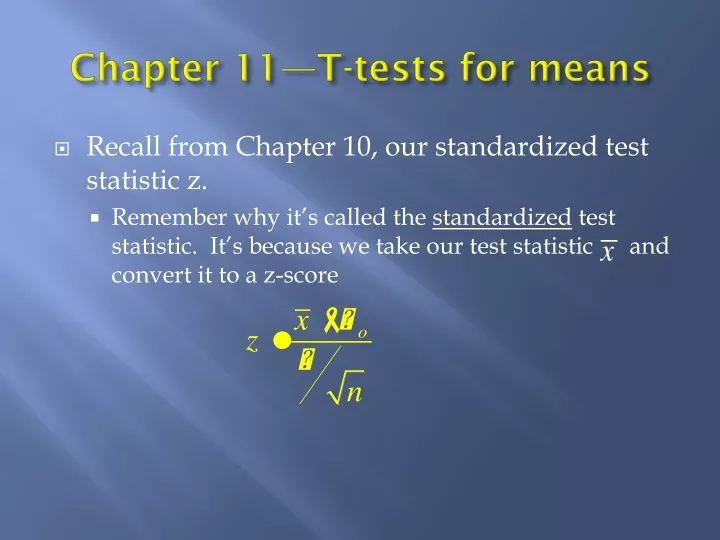
Chapter 11—T-tests for means. Recall from Chapter 10, our standardized test statistic z. Remember why it’s called the standardized test statistic. It’s because we take our test statistic and convert it to a z-score.

E N D
Chapter 11—T-tests for means • Recall from Chapter 10, our standardized test statistic z. • Remember why it’s called the standardized test statistic. It’s because we take our test statistic and convert it to a z-score
Remember the origin of our sampling distribution: It was what you get when you take all possible samples of a certain size, measure the mean of each sample, and place it in the forest of similar means. That gave you the distribution, whose mean was the same as our null hypothesis and whose standard deviation was • The problem is…nobody really knows σ.
Enter William Gossett • William Gosset figured a work-around for not knowing σ. By basing the standardized test statistic not on z, but on a family of curves called t, it became possible to use s, the sample standard deviation, for inference procedures. • The t-curves are based on “degrees of freedom,” which is n-1. (See tables inside the back cover of your textbook.
“Standard Error,” not Standard Deviation • What we used to call standard deviation of the sampling distribution, We now call Standard Error. s is sample standard deviation. This is not the last version of Standard Error we’ll see, but every time our measure of spread is based on sample data, it will be called Standard Error.
The t statistic (for one sample tests) It functions just like z did in Chapter 10, only now, use the tcdf function instead of normalcdf to get your p-value. Tcdf arguments: (left boundary of shaded area, right boundary, degrees of freedom)
t for confidence intervals The structure is just as we saw in Chapter 10. Get t* from the t-table inside the back cover of your book. In the table cross Confidence Level with Degrees of Freedom (which = n-1) Get s from 1-var stats using your data. When the time comes (Step 3 of a toolbox), you can use “T-Interval” under Stat—Test in your calculator.
The t curves • See page 618 in YMS. • Notice that the t curves are always thicker in the tails and shorter in the middle • Notice also that as degrees of freedom gets large, the t curve approaches the z curve. That means that as sample size gets larger and larger, you may as well use z! • There another implication: The t statistic works even with small sample sizes.
Conditions for using t • SRS • Population must be normal • (Notice—in Chapter 10, it was the sampling distribution that had to be normal. Now it’s the population) • SRS is the more important condition. • “Population normal” is actually quite non-critical.
Conditions for using t • “Population Normal”—Relax! Of course you don’t really know whether the population is normal, so instead you look for evidence of non-normality. Even then—the procedures are remarkably forgiving. See page 636. • If n<15, use t if data are close to normal, and there are no outliers. (Use NPP, histogram or stemplot) • If n at least 15, use t unless there are outliers or strong skew in the data • If n is big (40 or greater) you can safely use t even with clearly skewed data.
Group 1 Compare Average Response All Participants Random Assignment Group 2 Two-Sample Tests Think Chapter 5—Experimental Design. Remember the Random Comparative design?
Group 1 Compare Average Response All Participants Random Assignment Group 2 Two-Sample Tests What’s our Random Variable here? What would equal 0 if our null hypothesis is true? What’s our Null Hypothesis???? OMG!!!! All These Questions!!!
Group 1 Compare Average Response All Participants Random Assignment Group 2 Two-Sample Tests What’s our Random Variable here? ANSWER: The difference of the two means! What would equal 0 if our null hypothesis is true? ANSWER: The difference of the two means! What’s our Null Hypothesis? ANSWER: There is no difference between the two means!!
Two-Sample t-test for means • Our Null Hypothesis now is: There is no difference between the averages of the two groups: (or ) • Alternate Hypotheses can be any of these (Note that any of these could be expressed as “the difference is greater than zero, less than zero, or not equal to zero.”)
Back to Chapter 7 for a moment (Combining random variables) • Combine two normal sampling distributions through subtraction • What’s the mean? • What’s the standard deviation? • Take a peek at the equation sheet. Anything seem familiar?
Pooling What the heck is it, and when do you use it?
What is it? • Pooling is the idea of considering both populations in a two-sample test really to be part of the same population. • In other words, if Ho is is then we’re also asserting that • The two populations have the same variance, in other words. • In this situation, you can use df = n1+n2 – 2, and the “pooled” choice in your calculator. • (Reference: AMSCO p. 209)
On the other hand… • In other words, if Ho is some other number, then the the two populations are by definition different. • Assume different variance, or “unpooled.” • Use df = the lesser of n1 - 1 or n2 – 1. • Note: your textbook neglects this idea, but AMSCO is better on this point.