Download
1 / 45
450 likes | 592 Views
Photo-realistic Rendering and Global Illumination in Computer Graphics Spring 2012 Stochastic Path Tracing Algorithms. K. H. Ko School of Mechatronics Gwangju Institute of Science and Technology. Environment Map Illumination. Capturing Environment Maps

E N D
Photo-realistic Rendering and Global Illumination in Computer Graphics Spring 2012Stochastic Path Tracing Algorithms K. H. Ko School of Mechatronics Gwangju Institute of Science and Technology
Environment Map Illumination • Capturing Environment Maps • Environment maps usually represent real-world illumination conditions. • A light probe in conjunction with a digital camera or a digital camera equipped with a fisheye lens are the most common techniques for capturing environment maps.
Environment Map Illumination • Capturing Environment Maps • Light Probe • It is a practical way to acquire an environment map of a real environment. • A light probe is nothing more than a specular reflective ball that is positioned at the point where the incident illumination needs to be captured. • The light probe is subsequently photographed using a camera equipped with an orthographic lens. • Or alternatively, a large zoom lens can be used such that orthographic conditions are approximated as closely as possible.
Environment Map Illumination • Capturing Environment Maps • Light Probe • The center pixel in the recorded image of the light probe corresponds with a single incident direction. • This direction can be computed rather easily, since the normal vector on the light probe is known, and a mapping from pixel coordinates to incident directions can be used.
Environment Map Illumination • Capturing Environment Maps • Light Probe • A photograph of lithe light probe can results in a set of samples L(x<-Θ).
Environment Map Illumination • Capturing Environment Maps • Light Probe • The acquisition process is straightforward. However, there are a number of issues to be considered. • The camera will be reflected in the light probe and will be present in the photograph, thereby blocking light coming from directions directly behind the camera. • The use of a light probe does not result in a uniform sampling of directions over the hemisphere. Directions opposite the camera are sampled poorly, whereas directions on the same side of the camera are sampled densely.
Environment Map Illumination • Capturing Environment Maps • All directions sampled at the edge of the image of the light probe represent illumination from the same direction. Since the light probe has a small radius, these values may differ slightly. • Since the camera cannot capture all illumination levels due to its nonlinear response curve, a process of high dynamic range photography needs to be used to acquire an environment map that correctly represents radiance values.
Environment Map Illumination • Capturing Environment Maps • Light Probe • Some of the problems can be alleviated by capturing two photographs of the light probe 90 degrees apart. • The samples of both photographs can be combined into a single environment map.
Environment Map Illumination • Capturing Environment Maps • Fisheye Lens • An alternative for capturing an environment map is to make use of a camera equipped with a fisheye lens. • Two photographs taken from opposite view directions result in a single environment map as well. • Limitations • Good fisheye lenses can be very expensive and hard to calibrate. • Both images need to be taken in perfect opposite view directions, otherwise a significant set of directions will not be present in the photograph. • If the incident illumination of directions in only one hemisphere needs to be known instead of the full sphere of directions, the use of fisheye lens can be very practical.
Environment Map Illumination • Parameterization • When using environment maps in global illumination algorithms, they need to be expressed in some parameter space. • The effectiveness of how well environments maps can be sampled is dependent on the type of parameterization used. • In essence, this is the same choice one has to make when computing the rendering equation as an integral over the hemisphere.
Environment Map Illumination • Parameterization • Latitude-longitude parameterization • This is the same parameterization as the hemispherical coordinate system but extended to the full sphere of directions. • The advantage is an equal distribution of the tilt angle θ, but there is a singularity around both poles, which are represented as lines in the map. • Additional problems are that the pixels in the map do not occupy equal solid angles and that the Ф=0 and Ф=2π angles are not mapped continuously next to each other.
Environment Map Illumination • Parameterization • Projected-disk parameterization • It is also known as Nusselt embedding. • The hemisphere of directions is projected on a disk of radius 1. • The advantages are the continuous mapping of the azimuthal angle Ф, and the pole being a single point in the map. • However, the tilt angle θ is nonuniformly distributed over the map.
Environment Map Illumination • Parameterization • Projected-disk parameterization • A variant is the paraboloid parameterization, in which the tilt angle is distributed more evenly.
Environment Map Illumination • Parameterization • Concentric-map parameterization • The concentric map parameterization transforms the projected unit disk to a unit square. • This makes sampling of directions in the map easier and keeps the continuity of the projected-disk parameterizations.
Environment Map Illumination • Sampling Environment Maps • The direct illumination of a surface point due to an environment map can be expressed as follows: • The integrand contains the incident illumination on point x, coming from direction Ψ in the environment map.
Environment Map Illumination • Sampling Environment Maps • Other surfaces present in the scene might prevent the light coming from direction Ψ reaching x. • These surfaces might belong to other objects • The object to which x belongs can cast self-shadows onto x. • In these cases, a visibility term V(x,Ψ) has to be added:
Environment Map Illumination • Sampling Environment Maps • A straightforward application of Monte Carlo integration would result in the following estimator: • Here the different sampled direction Ψi are generated directly in the parameterization of the environment map using a PDF p(Ψ)
Environment Map Illumination • Sampling Environment Maps • Problems exist when trying to approximate this integral using Monte Carlo integration. • Integration domain • The environment map acting as a light source occupies the complete solid angle around the point to be shaded. • The integration domain of the direct illumination equation has a large extent, usually increasing variance.
Environment Map Illumination • Sampling Environment Maps • Problems exist when trying to approximate this integral using Monte Carlo integration. • Textured light source • Each pixel in the environment map represents a small solid angle of incident light. • The environment map can be considered as a textured light source. • The radiance distribution in the environment map can contain high frequencies or discontinuities. • Thereby it may increase variance and stochastic noise in the final image. • Especially when capturing effects such as the sun or bright windows, very high peaks of illumination values can be present in the environment map.
Environment Map Illumination • Sampling Environment Maps • Problems exist when trying to approximate this integral using Monte Carlo integration. • Product of environment map and BRDF • The integrand contains the product of the incident illumination Lmap and the BRDF fr. • The discontinuities and high-frequency effects present in the environment map. • A glossy or specular BRDF also contains very sharp peaks. • These peaks on the sphere or hemisphere of directions for both illumination values and BRDF values are usually not located at the same directions. • This makes it very difficult to design a very efficient same sheme that takes these features into account.
Environment Map Illumination • Sampling Environment Maps • Problems exist when trying to approximate this integral using Monte Carlo integration. • Visibility • If the visibility term is included, additional discontinuities are present in the integrand. • It might complicate an efficient sampling process.
Environment Map Illumination • Sampling Environment Maps • PDF p(Ψ)s that address such problems are presented. • Three categories for the PDFs. • PDFs based on the distribution of radiance values Lmap in the illumination map only, usually taking into account cos(Ψ,Nx) that can be pre-multiplied into the illumination map. • PDFs based on the BRDF fr, which are especially useful if the BRDF is of a glossy or specular nature • PDFs based on the product of both functions.
Environment Map Illumination • Methods for Constructing PDFs • Direct illumination map sampling • BRDF sampling • Sampling the product
Environment Map Illumination • Direct illumination map sampling • Transform the piecewise-constant pixel values into a PDF by computing the cumulative distribution in two dimensions and subsequently inverting it. • This typically results in a 2D look-up table, and the efficiency of the method is highly dependent on how fast this look-up table can be queried. • To simplify the environment map by transforming it to a number of well-selected point light sources. • Advantage: There is a consistent sampling of the environment map for all surface points to be shaded. • But it can possibly introduce aliasing artifacts, especially when using a low number of light sources.
Environment Map Illumination • BRDF sampling • The main disadvantage of constructing a PDF based only on the illumination map • The BRDF is not included in the sampling process but is left to be evaluated after the sampling directions have been chosen. • Problematic for specular and glossy BRDFs. • A PDF based on the BRDF will produce better results. • The BRDF can be sampled analytically. • But not possible in general except for a few well-constructed BRDFs. • The inverse cumulative distribution technique can be used.
Environment Map Illumination • Sampling the product • The best approach is to construct a sampling scheme based on the product of both the illumination map and the BRDF. • Possibly including the cosine and some visibility information as well. • Bidirectional importance sampling • It constructs a sampling procedure based on rejection sampling. • The disadvantage • It is difficult to predict exactly how many samples will be rejected and hence the computation time.
Indirect Illumination • Indirect Illumination • As oppose to direct illumination computations, this problem is usually much harder. • Indirect light might reach a surface point x from all possible directions. • It is very hard to optimize the indirect illumination computations along the same lines as was done for direct illumination. • Indirect illumination consists of the light reaching a target point x after at least one reflection at an intermediate surface between the light sources and x. • It is a very important component of the total light distribution in a scene. • Usually takes the largest amount of work in any global illumination algorithm.
Indirect Illumination • Uniform Sampling for Indirect Illumination • The indirect illumination contribution to L(x->Θ) is • The integrand contains the reflected radiances Lr from other points in the scene. • They are themselves composed of a direct and indirect illumination part.
Indirect Illumination • Uniform Sampling for Indirect Illumination • This integral cannot be reformulated to a smaller integration domain. • Lr has (in a closed environment) a nonzero value for all (x,Ψ) pairs. • So the entire hemisphere needs to be considered as the integration domain and needs to be sampled accordingly. • The most general Monte Carlo procedure to evaluate the indirect illumination is to use an arbitrary, hemispherical PDF p(Ψ) and to generate N random directions Ψi. • The estimator:
Indirect Illumination • Uniform Sampling for Indirect Illumination • To evaluate this estimator, we need to do • Evaluate the BRDF • Evaluate the cosine term, • Trace a ray from x in the direction of Ψi • Evaluate the reflected radiance Lr(r(x,Ψi)-> -Ψi)
Indirect Illumination • Uniform Sampling for Indirect Illumination • The evaluation of Lr shows the recursive nature of indirect illumination. • This reflected radiance at r(x,Ψi) can be split again into a direct and indirect contribution. • The recursive evaluation can be stopped using Russian roulette. • Generally, the local hemispherical reflectance is used as an appropriate absorption probability.
Indirect Illumination • Uniform Sampling for Indirect Illumination Paths generated during indirect illumination computations. Shadow rays for direct illumination are shown as dashed lines.
Indirect Illumination • Importance Sampling for Indirect Illumination • The simplest choice for p(Ψ) is a uniform PDF p(Ψ)=1/2π. • Directions are sampled proportional to solid angles. • It is easy and straightforward to implement. • Noise in the resulting picture will be caused by variations in the BRDF and cosine evaluations, and variations in the reflected radiance Lr at the distant points.
Indirect Illumination • Importance Sampling for Indirect Illumination • Uniform sampling over the hemisphere does not take into account any knowledge we might have about the integrand in the indirect illumination integral. • In order to reduce noise, some form of importance sampling is needed.
Indirect Illumination • Importance Sampling for Indirect Illumination • Construction of a hemispherical PDF proportional to any of the following factors: • The cosine factor cos(Ψi,Nx) • The BRDF fr(x,Θ<->Ψi) • The incident radiance field Lr(r(x,Ψi) • A combination of any of the above.
Indirect Illumination • Cosine Sampling • Sampling directions proportional to the cosine lobe around the normal Nx prevents too many directions from being sampled near the horizon of the hemisphere where cos(Ψ,Nx) equals 0. • The noise is expected to decrease since we reduce the probability of directions being generated that contribute little to the final estimator.
Indirect Illumination • Cosine Sampling • The PDF becomes • If we also assume that the BRDF fr is diffuse at x, we obtain the following estimator: • The only sources of noise are variations in the incident radiance field.
Indirect Illumination • BRDF Sampling • When sampling directions Ψ over the hemisphere proportional to the cosine factor, we do not take into account that due to the nature of the BRDF at x, some directions contribute much more to the value of Lindirect(x->Θ). • Ideally, directions with a high BRDF value should be sampled more often. • BRDF sampling is a good noise-reducing technique when a glossy or highly specular BRDF is present. • It diminishes the probability that directions are sampled where the BRDF has a low or zero value.
Indirect Illumination • BRDF Sampling • However, only for a few selected BRDF models, it is possible to sample exactly proportional to the BRDF. • Better approach • Try to sample proportional to the product of the BRDF and the cosine term. • Analytically this is even more difficult to do. • Usually, a combination with rejection is needed to sample according to such a PDF.
Indirect Illumination • An alternative method • Build a numerical table of the cumulative probability function and generate directions using this table. • Time consuming • The PDF value will not be exactly equal to the product of BRDF and cosine factors. • But a significant variance reduction can be achieved.
Indirect Illumination • A perfect specular material can be modeled using a Dirac impulse for the BRDF. • Sampling the BRDF simply means we only have one possible direction from which incident radiance contributes to the indirect illumination. • Such Dirac BRDF is difficult to fit in a Monte Carlo sampling framework. • A special evaluation procedure usually needs to be written.
Indirect Illumination • Proportional BRDF Sampling • Consider the modified Phong BRDF • Diffuse and glossy parts • The indirect illumination integral can now be split into two parts, according to those terms of the BRDF:
Indirect Illumination • Proportional BRDF Sampling • Sampling this total expression proceeds as follows: • A discrete PDF is constructed with three events, with respective probabilities q1, q2, and q3 (q1+q2+q3=1). • The three events correspond to deciding which part of the illumination integral to sample. • The last event can be used as an absorption. • Ψi is then generated using either p1(Ψ) or p2(Ψ), two PDFs that correspond, respectively to the diffuse and glossy part of the BRDF.
Indirect Illumination • Proportional BRDF Sampling • Sampling this total expression proceeds as follows: • The final estimator for a sampled direction Ψi is then equal to:
Indirect Illumination • Proportional BRDF Sampling • An alternative is to consider the sampled direction as part of a single distribution and evaluate the total indirect illumination integral. • The generated directions will have a subcritical distribution q1p1(Ψ)+q2p2(Ψ). • The corresponding primary estimator is