Download
1 / 41
410 likes | 501 Views
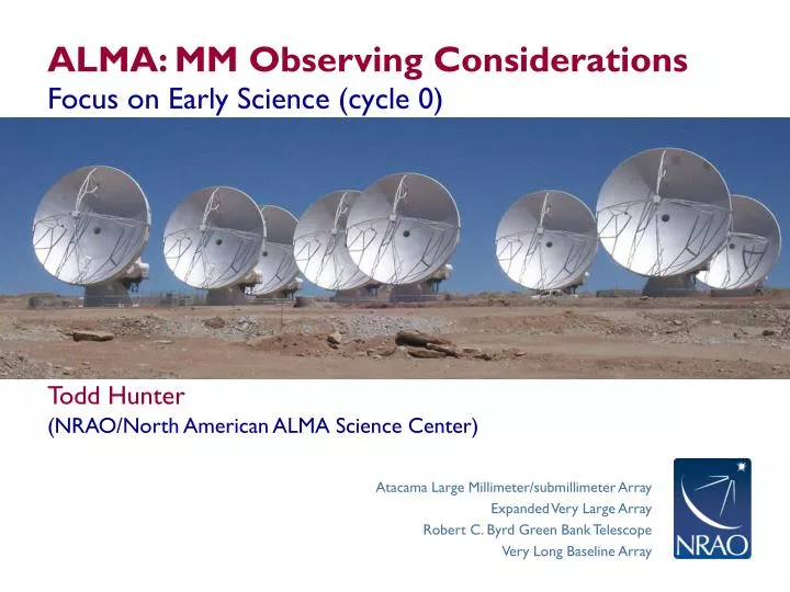
ALMA: MM Observing Considerations. Focus on Early Science (cycle 0). Todd Hunter. (NRAO/North American ALMA Science Center). Overview of Talk. Perspective: Getting time on ALMA will be competitive! The math: only ~600 hours for ES cycle 0

E N D
ALMA: MM Observing Considerations Focus on Early Science (cycle 0) • Todd Hunter • (NRAO/North American ALMA Science Center)
Overview of Talk • Perspective: Getting time on ALMA will be competitive! • The math: only ~600 hours for ES cycle 0 • at ~6 hours per project ~100 projects split over the world • Motivation: While ALMA is for everyone, a technical justification is required for each proposal, so you need to know some of the details of how the instrument works • Goal: Do the best job you can to match your science to ALMA’s capabilities
Sky coverage available • ALMA is at a latitude of -23 degrees Southern sky! • Antenna elevation limit is technically 3 degrees • But in practice, atmospheric opacity will cause significant degradation with lower elevation most severe at higher frequencies Maximum length of observation for Northern sources (hrs) Note: This table does not account for shadowing, which further impedes low elevation observations in compact configurations.
Receiver Bands Available 3 mm 1.3 mm 0.87 mm 0.45 mm • Only 4 of 8 bands are available for Early Science, all with dual linear polarization feeds • Only 3 receiver bands can be “ready” at one time (i.e. amplifiers powered on and stable temperature achieved). Required lead time to stabilize a new band is about 20 minutes. • With configurations of ~125m and ~400m, approximately matched resolution is possible between Bands 3 and 7, or between Bands 6 and 9 • Matched resolution can be critical, for example to measure the SEDs of resolved sources.
Atmospheric Opacity (PWV = Precipitable Water Vapor) O3 O2 H2O H2O H2O H2O
http://www.eso.org/sci/facilities/alma/observing/tools/etc Sensitivity calculator np = # polarizations N = # antennas Δν= channel width Δt = total time
Choosing your bands – I(constructed from sensitivity calculator) NOTE: For 8 GHz continuum bandwidth divide by √2
Choosing your bands - II (S/N=1 at 100 GHz)
Correlator Modes, Spectral Resolution, Spectral Coverage - I • Receivers are sensitive to two separate ranges of sky frequency: sidebands • Each antenna has 4 digitizers which can each sample 2 GHz of bandwidth • These 2 GHz chunks are termed basebands, and can be distributed among the sidebands (in ES: either all four in one, or two in both as shown below) For Bands 3 & 7 Local Oscillator Frequency (NOTE: In Band 9, you can also have 1 or 3 basebands in a sideband.)
Correlator Modes, Spectral Resolution, Spectral Coverage - II **For Bands 3 & 7 Spectral windows • In order to collect data, you need to set up a spectral window within one (or more) basebands. • In Early Science, only 4 spectral windows are available, i.e. one per baseband, and all must have the same resolution and bandwidth • **Note: exact spacing between sidebands and sideband widths vary from band to band – OT will show correct one for each band
Correlator Modes and Spectral Resolution Typical purposes: Spectral scans Targeted imaging of moderately narrow lines: cold clouds / protoplanetary disks “Continuum” or broad lines • These numbers are per baseband (you can use up to 4 basebands) • Usually want to have several channels across narrowest line • Note that the resolution is ~ 2*channel width (Hanning) • The required spectral resolution typically needs to be justified as does the number of desired spectral windows
Spectral Lines in the ALMA bands http://www.splatalogue.net (large subset also available in OT)
Spectral lines in the ALMA bands SMA spectrum of Arp 220 (Band 6) (Martin et al. 2011)
Image Quality • Sensitivity is not enough! Image quality also depends on UV coverage and density of UV samples • Image fidelity is improved when high density regions of UV coverage are well matched to source brightness distribution • The required DYNAMIC RANGE can be more important than sensitivity • ALMA OT currently has no way to specify required image quality, but you can request more time in the Technical Justification
Dirty Beam Shape and N Antennas 2 Antennas (Image sequence taken from Summer School lecture by D. Wilner)
Dirty Beam Shape and N Antennas 3 Antennas
Dirty Beam Shapeand N Antennas 4 Antennas
Dirty Beam Shape and N Antennas 5 Antennas
Dirty Beam Shape and N Antennas 6 Antennas
Dirty Beam Shape and N Antennas 7 Antennas
Dirty Beam Shape and N Antennas 8 Antennas
Dirty Beam Shape and N Antennas 8 Antennas x 6 Samples
Dirty Beam Shape and N Antennas 8 Antennas x 30 Samples
Dirty Beam Shape and N Antennas 8 Antennas x 60 Samples
Dirty Beam Shape and N Antennas 8 Antennas x 120 Samples
Dirty Beam Shape and N Antennas 8 Antennas x 240 Samples
Dirty Beam Shape and N Antennas 8 Antennas x 480 Samples
Effects of UV Coverage 5σ 5σ 10σ 15σ 20σ Note improved uv-coverage with time for same config.
Choose Single Field or Mosaic • Example: SMA 1.3 mm observations: 5 pointings • Primary beam ~1’ • Resolution ~3” 3.0’ ALMA 1.3mm PB ALMA 0.85mm PB CFHT 1.5’ In ES, the number of pointings will <= 50. Petitpas et al.
Maximum Angular Scale • Smooth structures larger than MAS are completely resolved out • Begin to lose total recovered flux for objects on the order of half MAS
Sensitivity and Brightness Temperature • There will be a factor of 10 difference in brightness temperature sensitivity between the 2 configurations offered in Early Science. Very important to take into account for resolved sources. Example: 1 minute integration at 230 GHz with 1 km/sec channels:
Observatory Default Calibration • Need to measure and remove the (time-dependent and frequency-dependent) atmospheric and instrumental variations. • Set calibration to system-defined calibration unless you have very specific requirements for calibration (which then must be explained in the Technical Justification). Defaults include (suitable calibrators are chosen at observation time): • Pointing, focus, and delay calibration • Phase and amplitude gain calibration • Absolute flux calibration • Bandpass calibration • System Temperature calibration • Water-vapor radiometry correction
ALMA Calibration Device Two-temperature load system (100C & ambient) maneuvered by robotic arm (shown in a Melco antenna below) Tsys≈Tatm(et -1) + Trxet t = to sec(el)
Atmospheric phase fluctuations Variations in the amount of precipitable water vapor (PWV) cause phase fluctuations, which are worse at shorter wavelengths (higher frequencies), and result in: Low coherence (loss of sensitivity) Radio “seeing”, typically 0.1-1² at 1 mm Anomalous pointing offsets Anomalous delay offsets You can observe in apparently excellent submm weather (in terms of transparency) and still have terrible “seeing” i.e. phase stability. Patches of air with different water vapor content (and hence index of refraction) affect the incoming wave front differently.
Phase correction methods Fast switching: used at the EVLA for high frequencies and will be used at ALMA. Choose cycle time, tcyc, short enough to reduce frmsto an acceptable level. Calibrate in the normal way. • Traditional calibrators (quasars) are more scarce at high frequency • But ALMA sensitivity is high, even on a per baseline basis • Key will be calibrator surveys (probably starting with ATCA survey)
Phase correction methods Fast switching: used at the EVLA for high frequencies and will be used at ALMA. Choose cycle time, tcyc, short enough to reduce frmsto an acceptable level. Calibrate in the normal way. However, the atmosphere often varies faster than the timescale of Fast Switching. The solution for ALMA is the WVR system. Water Vapor Radiometry (WVR) concept: measure the rapid fluctuations in TBatm with a radiometer at each antenna, then use these measurements to derive changes in water vapor column (w) and convert these into phase corrections using: Δfe» 12.6 p Δw / l
ALMA WVR System Installed on every antenna Two different baselines Jan 4, 2010 Data WVR Residual • There are 4 “channels” flanking the peak of the 183 GHz water line • Matching data from opposite sides are averaged • Data taken every second, and are written to the ASDM (science data file) • The four channels allow flexibility for avoiding saturation • Next challenges are to perfect models for relating the WVR data to the correction for the data to reduce residual phase noise prior to performing the traditional calibration steps.
Tests of ALMA WVR System 600m baseline, Band 6, Mar 2011 (red=raw data, blue=corrected)
Phase correction methods Fast switching: used at the EVLA for high frequencies and will be used at ALMA. Choose cycle time, tcyc, short enough to reduce frmsto an acceptable level. Calibrate in the normal way. Water Vapor Radiometry: measure rapid fluctuations in TBatm with a radiometer, then use these to derive changes in water vapor column (w) and convert these into phase corrections using:Δfe» 12.6pΔw/l Phase transfer:alternate observations at low frequency (calibrator) and high frequency (science target), and transfer scaled phase solutions from low to high frequency. Can be tricky, requires well characterized system due to differing electronics at the frequencies of interest. Self-calibration: possible for bright sources. Need S/N per baseline of a few on short times scales (typically a few seconds).
Future Capabilities • Better sensitivity and image fidelity: • Imaging fidelity ~10x better, Sensitivity > 3x better • Fantastic “snapshot” uv-coverage (50 x 12m antennas = 1225 baselines) • Higher angular resolution: • baselines ~15km, matched beams possible in all bands • Better imaging of resolved objects and mosaics • TPA: four additional 12m antennas with subreflector nutators • ACA: Atacama Compact configuration 12 x 7m antennas • “On-the-Fly” mosaics: quickly cover larger areas of sky • More receiver bands: 4, 8, 10 (2mm, 0.7mm, 0.35mm) • Polarization: magnetic fields and very high dynamic range imaging • “Mixed” correlator modes (simultaneous wide & narrow, see A&A 462, 801) • ALMA development program studies just beginning • mm VLBI, more receiver bands • Higher data rates
www.almaobservatory.org The Atacama Large Millimeter/submillimeter Array (ALMA), an international astronomy facility, is a partnership among Europe, Japan and North America, in cooperation with the Republic of Chile. ALMA is funded in Europe by the European Organization for Astronomical Research in the Southern Hemisphere, in Japan by the National Institutes of Natural Sciences (NINS) in cooperation with the Academia Sinica in Taiwan and in North America by the U.S. National Science Foundation (NSF) in cooperation with the National Research Council of Canada (NRC). ALMA construction and operations are led on behalf of Europe by ESO, on behalf of Japan by the National Astronomical Observatory of Japan (NAOJ) and on behalf of North America by the National Radio Astronomy Observatory (NRAO), which is managed by Associated Universities, Inc. (AUI). AAS217: Special Session