Download
1 / 30
300 likes | 447 Views
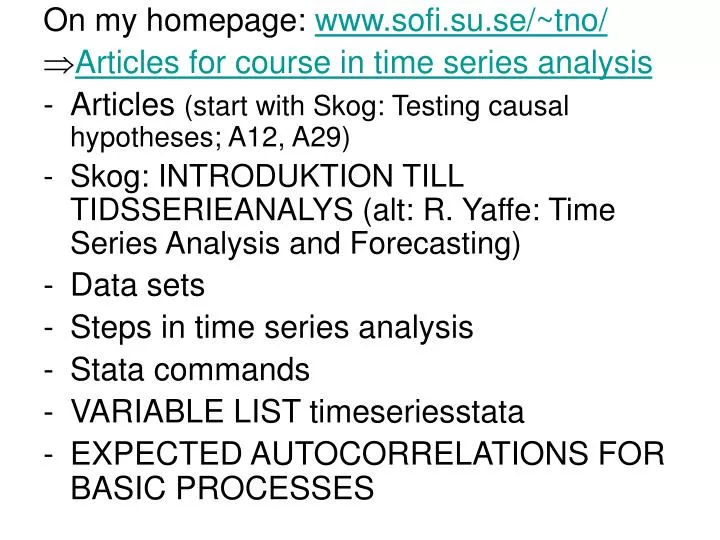
On my homepage: www.sofi.su.se/~tno/ Articles for course in time series analysis Articles (start with Skog: Testing causal hypotheses; A12, A29) Skog: INTRODUKTION TILL TIDSSERIEANALYS (alt: R. Yaffe: Time Series Analysis and Forecasting) Data sets Steps in time series analysis

E N D
On my homepage: www.sofi.su.se/~tno/ • Articles for course in time series analysis • Articles (start with Skog: Testing causal hypotheses; A12, A29) • Skog: INTRODUKTION TILL TIDSSERIEANALYS (alt: R. Yaffe: Time Series Analysis and Forecasting) • Data sets • Steps in time series analysis • Stata commands • VARIABLE LIST timeseriesstata • EXPECTED AUTOCORRELATIONS FOR BASIC PROCESSES
Course design • Introductions to topics in time series analysis and examples of applications • Computer exercises using available data sets (or your own). Stata 10 (SPSS 13) • Course requirement: perform and report an analysis following ” Steps in time series analysis”
Overview: topics • Questions addressed by time series analysis • Pros and cons • Important pitfalls • Structural shift • Impact-analysis • Natural experiment • Comparative analyses • Triangulation; integration of results from micro- & macro level
Questions addressed by time series analysis (TSA) • Micro data: explain individual variation: why do some individuals become criminals (alcohol abusers) • Macro data: explain trends on population level: what causes variation in crime rates (prevalence of alcohol abuse)? • A certain X (genes) may be important on micro level but not on macro level (obesity) • Explain trends in Y vs estimate effects of X (Example: alcohol and total mortality)
Examples of applications of TSA • Prices – consumption • Unemployment – inflation • Alcohol and various outcomes (cirrhosis, violence, suicide) • Economic growth and mortality • Impact-analyses: Saturday opening, law changes, strikes
Advantages • Cheap data • Avoids selection effects • Less problem with reversed causation • Policy relevant questions
Drawbacks • Easy to obtain spurious relationships • Easy to manipulate, eg. with time-lags same data may give different results scepticism from referees • But: ARIMA (Autoregressive Integrated Moving Average) gives more accurate results
Important pitfalls • Warning for trend comparisons • Outliers • Omitted lag-effect
Alcohol consumption (down) and real wages (up), 1861-1914, Sweden
Instead of estimating the relationship between wages and consumption from the trending raw data: Yt = b*Xt We should do the analysis on the differenced series: Yt = b* Xt därYt = Yt - Yt -1 Differencing is a simple and efficient way to remove trends
Example of outlier:Divorce rate (X-axis) and cirrhosis mortality (Y-axis)
Alcohol consumption (solid) and alcohol related mortality.Raw data (left),weighted consn (right)
Popham vs. Skog (1980) Liver cirrhosis epidemiology: some methodological problems, British Journal of Addiction
Reversed causation Micro data: correlation between alcohol abuse and sickness absence. Hard to determine what comes first. Macro data: correlation between alcohol/capita (X1) and sickness absence rate (X2) X2 cannot cause X1 (too few people)
Alcohol suicide? Micro data: Alcohol abusers have an elevated suicide risk. Problem: selection Mental problems Suicide Alcohol
Alcohol suicide? Macro data: No selection problem Prevalence mental problems Suicide rate Alcohol/capita
Elimination of selection bias by aggregation Micro model: Yit = Ci + bXit+eit Ci is stable over time. Estimate of b is biased if Ci is correlated withXit Macro model: Yt = C+ bXt+et Now C is a constant and by definition uncorrelated withXt . Example: Y=violence, C=aggression, X= alcohol
Alcohol protects against IHD (heart diesease)? Micro data: Negative correlation alcohol-IHD. Problem: selection: Blood pressure - + Alcohol IHD-risk -?
Alcohol protects against IHD? Macro data: no selection problem Prevalence high blood pressure + Alcohol/cap IHD-rate -?
Unemployment suicide? Micro data: Unemployed have an elevated suicide risk. Problem: selection Mental problems Unemployment Suicide risk
Unemployment suicide? Macro data: No selection problem (if the cross at the left arrow isn’t true we have omitted variable bias) Prevalence mental problems % Unemployed Suicide rate
Alcohol suicide? Macro data: New problem: omitted variable bias % Unemployed - + Suicide rate Alcohol/capita +
Omitted variable bias: remedies • Include the variable (% unemployed) • Natural experiment: choose a period when X (alcohol) changes much due to causes (rationing) that don’t affect Y • Example: Denmark 1917, when alcohol consumption decreased strongly due to war restrictions (Data: Danmarkww1.dat)
O-J Skog: Alcohol & suicide in Denmark(Addiction 1993) Illustatrates several advantages of TSA: • Research economy: 3*14 observations • No selection bias • No omitted variable bias Strong evidence value
Number of observations for TSA • Normally >30 • Strong variation in X few observations is enough