Download
1 / 24
240 likes | 473 Views
CPU Management. CT213 – Computing Systems Organization. Content . Process scheduler organization Scheduler types: Non-preemptive Preemptive Scheduling algorithms FCFS (First Come First Served) SRTN (Shortest Remaining Time Next)/ SJF Shortest Job First Time slice (Round Robin)

E N D
CPU Management CT213 – Computing Systems Organization
Content • Process scheduler organization • Scheduler types: • Non-preemptive • Preemptive • Scheduling algorithms • FCFS (First Come First Served) • SRTN (Shortest Remaining Time Next)/ SJF Shortest Job First • Time slice (Round Robin) • Priority based preemptive scheduling • MLQ (Multiple Level Queue) • MLQF (Multiple Level Queue with Feedback) • BSD Unix scheduler
Scheduling • Is the mechanism, part of the process manager, that handles the removal of the running process from the CPU and the selection of another process • The selection of another process is based on a particular strategy • It is responsible for multiplexing processes on the CPU; when is the time for the running process to be removed from the CPU (in a ready or suspended state), a different process is selected from the set of process in the ready state • Policy – determines when the process is removed and what next process takes the control of the CPU • Mechanism – how the process manager knows it is the time to remove the current process and how a process is allocated/de-allocated from the CPU
Scheduler organization • When a process is changed in the ready state, the enqueuer places a pointer to the process descriptor into a ready list • Context switcher saves the content of all processor registers of the process being removed into the process’ descriptor, whenever the scheduler switches the CPU from executing a process to executing another • Voluntary context switch • Involuntary context switch • The dispatcher is invoked after the current process has been removed from the CPU; the dispatcher chooses one of the processes enqueued in the ready list and then allocates CPU to that process by performing another context switch from itself to the selected process
Scheduler types • Cooperative scheduler (voluntary CPU sharing) • Each process will periodically invoke the process scheduler, voluntarily sharing the CPU • Each process should call a function that will implement the process scheduling. • yield (Pcurrent, Pnext) (sometime implemented as an instruction in hardware), where Pcurrent is an identifier of the current process and the Pnext is an identifier of the next process) • Preemptive scheduler (involuntary CPU sharing) • The interrupt system enforces periodic involuntary interruption of any process’s execution; it can force a process to involuntarily execute a yield type function (or instruction) • This is done by incorporating an interval timer device that produces an interrupt whenever the time expires
Cooperative scheduler • Possible problems: • If the processes are not voluntarily cooperate with the others • One process could keep the process forever
Preemptive scheduler • A programmable interval timer will cause an interrupt to run every K clock tics of an interval timer, thus causing the hardware to execute the logical equivalent of a yield instruction to invoke the interrupt handler • The interrupt handler for the timer interrupt will call the scheduler to reschedule the processor without any action on the part of the running process • The scheduler is guaranteed to be invoked once every K clock ticks • Even if a given process will execute an infinite loop, it will not block the execution of the other processes IntervalTimer{ InterruptCount = InterrptCount -1; if (InterruptCount <=0){ InterruptRequest = TRUE InterruptCount = K; } } SetInterval(<programableValue>{ K = prgrammableValue; InterruptCount = K; }
Performance elements • Having a set of processes P={pi, 0<=i<n} • Service time, τ(pi) – the amount of time a process needs to be in active/running state before completes • Wait time, W(pi) – the time the process waits in the ready state before its first transition in the active state • Turn around time TTRnd(pi) – the amount of time between the moment a process enters the ready state and the moment the process exits the running state for the last time • Those elements are used to measure the performance of each scheduling algorithm
Selection strategies • Non preemptive strategies • Allow any process to run to completion once it has been allocated the control of the CPU • A process that gets the control of the CPU, releases the CPU whenever it ends or when it voluntarily give the control of the CPU • Preemptive strategies • The highest priority process among all ready processes is allocated the CPU • All lower priority processes are made to yield to the highest priority process whenever requests the CPU • The scheduler is called every time a process enters the ready queue as well as when an interval timer expires and a time quantum has elapsed • It allows for equitable resource sharing among processes at the expense of overloading the system
Scheduling algorithms • FCFS (First Come First Served) • SRTN (Shortest Remaining Time Next)/ SJF Shortest Job First • Time slice (Round Robin) • Priority based preemptive scheduling • MLQ (Multiple Level Queue) • MLQF (Multiple Level Queue with Feedback)
First Come First Served • Non-preemptive algorithm • This scheduling strategy assigns priority to processes in the order in which they request the processor • The priority of a process is computed by the enqueuer by time stamping all incoming processes and then having the dispatcher to select the process that has the oldest time stamp • Alternative implementation consists of having the ready list organized as a FIFO data structure (where each entry points to a process descriptor); the enqueuer adds processes to the tail of the queue and the dispatcher removes processes from the head of the queue • Easy to implement • it is not widely used, because the turn around time and the waiting time for a given process are not predictable.
FCFS example • Average turn around time: • TTRnd = (350 +475 +950 + 1200 + 1275)/5 = 850 • Average wait time: • W = (0 + 350 +475 + 950 + 1200)/5 = 595 TTRnd(pi)
Shortest Job First • There are non-preemptive and preemptive variants • It is an optimal algorithm from the point of view of average turn around time; it minimizes the average turn around time • Preferential service of short jobs • It requires the knowledge of the service time for each process • In the extreme case, where the system has little idle time, the processes with large service time will never be served • In the case where it is not possible to know the service time for each process, this is estimated using predictors • Pn = aOn-1 + (1-a)Pn-1 where • On-1 = previous service time • Pn-1 = previous predictor • a is within [0,1] range • If a = 1 then Pn-1 is ignored • Pn is dependent upon the history of the process evolution
SJF example • Average turn around time: • TTRnd = (800 + 200 +1275 + 450 + 75)/5 = 560 • Average wait time: • W = (450 + 75 +800 + 200 + 0)/5 = 305 TTRnd(pi)
Time slice (Round Robin) • Preemptive algorithm • Each process gets a time slice of CPU time, distributing the processing time equitably among all processes requesting the processor • Whenever the time slice expires, the control of the CPU is given to the next process in the ready list; the process being switched is placed back into the ready process list • It implies the existence of a specialized timer that measures the processor time for each process; every time a process becomes active, the timer is initialized • It is not well suited for long jobs, since the scheduler will be called multiple times until the job is done • It is very sensitive to the size of the time slice • Too big – large delays in response time for interactive processes • Too small – too much time spent running the scheduler • Very big – turns into FCFS • The time slice size is determined by analyzing the number of the instructions that the processor can execute in the give time slice.
Time slice (Round Robin) example • Average turn around time: • TTRnd = (1100 + 550 + 1275 + 950 + 475)/5 = 870 • Average wait time: • W = (0 + 50 + 100 + 150 + 200)/5 = 100 • The wait time shows the benefit of RR algorithm in the terms of how quickly a process receives service Time slice size is 50, negligible amount of time for context switching
RR scheduling with overhead example • Average turn around time: • TTRnd = (1320 + 660 + 1535 + 1140 + 565)/5 = 1044 • Average wait time: • W = (0 + 60 + 120 + 180 + 240)/5 = 120 Time slice size is 50, 10 units of time for context switching
Priority based scheduling (Event Driven) • Both preemptive and non-preemptive variants • Each process has an externally assigned priority • Every time an event occurs, that generates process switch, the process with the highest priority is chosen from the ready process list • There is the possibility that processes with low priority will never gain CPU time • There are variants with static and dynamic priorities; the dynamic priority computation solves the problem with processes that may never gain CPU time (the longer the process waits, the higher its priority becomes) • It is used for real time systems
Priority based schedule example • Average turn around time: • TTRnd = (350 + 425 + 900 + 1025 + 1275)/5 = 795 • Average wait time: • W = (0 + 350 + 425 + 900 + 1025)/5 = 540 Highest priority corresponds to highest value
Multiple Level Queue scheduling • Complex systems have requirements for real time, interactive users and batch jobs, therefore a combined scheduling mechanism should be used • The processes are divided in classes • Each class has a process queue, and it has assigned a specific scheduling algorithm • Each process queue is treated according to a queue scheduling algorithm: • Each queue has assigned a priority • As long as there are processes in a higher priority queue, those will be serviced
MLQ example • 2 queues • Foreground processes (highest priority) • Background processes (lowest priority) • 3 queues • OS processes and interrupts (highest priority, serviced ED) • Interactive processes (medium priority, serviced RR) • Batch jobs (lowest priority, serviced FCFS)
Multiple Level Queue with feedback • Same with MLQ, but the processes could migrate from class to class in a dynamic fashion • Different strategies to modify the priority: • Increase the priority for a given process during the compute intensive paths (in the idea to that the user needs larger share of the CPU to sustain acceptable service) • Decrease the priority for a given process during the compute intensive paths (in the idea that the user process is trying to get more CPU share, which may impact on the other users) • If a process is giving the CPU before its time slice expires, then the process is assigned to a higher priority queue • During the evolution to completion, a process may go through a number of different classes • Any of the previous algorithms may be used for treating a specific process class.
Practical example: BSD UNIX scheduling • MLQ with feedback approach – 32 run queues • 0 through 7 for system processes • 8 through 31 for processes executing in user space • The dispatcher selects a process from the queue with highest priority; within a queue, RR is used, therefore only processes in highest priority queue can execute; the time slice is less than 100us • Each process has an external priority (used to influence, but not solely determine the queue where the process will be placed after creation) • The sleep routine has the same effect as a yield instruction; when called from a process, the scheduler is called to dispatch a new process; otherwise the scheduler is called as result of a trap instruction execution or the occurrence of an interrupt
References • “Operating Systems – A modern perspective”, Garry Nutt, ISBN 0-8053-1295-1