Download
1 / 60
640 likes | 687 Views
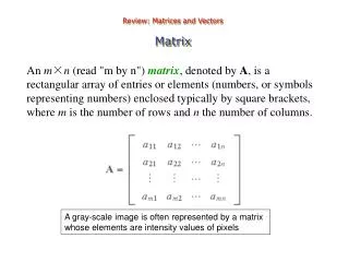
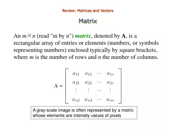
Review: Matrices and Vectors. Matrix. An m × n (read "m by n") matrix , denoted by A , is a rectangular array of entries or elements (numbers, or symbols representing numbers) enclosed typically by square brackets, where m is the number of rows and n the number of columns.

E N D
Review: Matrices and Vectors Matrix An m×n (read "m by n") matrix, denoted by A, is a rectangular array of entries or elements (numbers, or symbols representing numbers) enclosed typically by square brackets, where m is the number of rows and n the number of columns. A gray-scale image is often represented by a matrix whose elements are intensity values of pixels
Review: Matrices and Vectors Matrix Definitions (Con’t) • A issquare if m= n. • A isdiagonal if all off-diagonal elements are 0, and not all diagonal elements are 0. • A is the identity matrix ( I ) if it is diagonal and all diagonal elements are 1. • A is the zero or null matrix ( 0 ) if all its elements are 0. • The trace of A equals the sum of the elements along its main diagonal. • Two matrices A and B are equal iff the have the same number of rows and columns, and aij = bij .
Review: Matrices and Vectors Matrix Definitions (Con’t) • The transposeAT of an m×n matrix A is an n×m matrix obtained by interchanging the rows and columns of A. • A square matrix for which AT=A is said to be symmetric. • Any matrix X for which XA=I and AX=I is called the inverse of A. • Let c be a real or complex number (called a scalar). The scalar multiple of c and matrix A, denoted cA, is obtained by multiplying every elements of A by c. If c = 1, the scalar multiple is called the negative of A.
Review: Matrices and Vectors Block Matrix A block matrix is a matrix that is defined using smaller matrices, called blocks Example Exercise (Hadamard Matrix)
Review: Matrices and Vectors Block Matrix (con’t) H=256 W=256 divided into 1024 88 block matrices in JPEG compression
Review: Matrices and Vectors Row and Column Vectors A column vector is an m × 1 matrix: A row vector is a 1 × n matrix: A column vector can be expressed as a row vector by using the transpose:
Review: Matrices and Vectors Vector Norms There are numerous norms that are used in practice. In our work, the norm most often used is the so-called 2-norm, which, for a vector x in real m, space is defined as which is recognized as the Euclidean distance from the origin to point x; this gives the expression the familiar name Euclidean norm. The expression also is recognized as the length of a vector x, with origin at point 0. From earlier discussions, the norm also can be written as
Review: Matrices and Vectors Some Basic Matrix Operations • The sum of two matrices A and B (of equal dimension), denoted A + B, is the matrix with elements aij + bij. • The difference of two matrices, A B, has elements aij bij. • The product, AB, of m×n matrix A and n×q matrix B, is an m×q matrix C whose (i,j)-th element is formed by multiplying the entries across the ith row of A times the entries down the jth column of B; that is,
Review: Matrices and Vectors Some Basic Matrix Operations (Con’t) The inner product (also called dot product) of two vectors is defined as Note that the inner product is a scalar.
Review: Matrices and Vectors Inner Product The Cauchy-Schwartz inequality states that Another well-known result used in the book is the expression where is the angle between vectors x and y. From these expressions it follows that the inner product of two vectors can be written as Thus, the inner product can be expressed as a function of the norms of the vectors and the angle between the vectors.
Review: Matrices and Vectors Geometric Intuition
Review: Matrices and Vectors Orthogonality and Orthonormality From the preceding results, two vectors in m are orthogonal if and only if their inner product is zero. Two vectors are orthonormal if, in addition to being orthogonal, the length of each vector is 1. From the concepts just discussed, we see that an arbitrary vector a is turned into a vector an of unit length by performing the operation an = a/||a||. Clearly, then, ||an|| = 1. A set of vectors is said to be an orthogonal set if every two vectors in the set are orthogonal. A set of vectors is orthonormal if every two vectors in the set are orthonormal.
Review: Matrices and Vectors Some Important Aspects of Orthogonality Let B = {v1,v2,…,vn } be an orthogonal or orthonormal basis in the sense defined in the previous section. Then, an important result in vector analysis is that any vector v can be represented with respect to the orthogonal basis B as where the coefficients are given by
Review: Matrices and Vectors Geometric Example
Review: Probability and Random Variables Sets and Set Operations Probability events are modeled as sets, so it is customary to begin a study of probability by defining sets and some simple operations among sets. A set is a collection of objects, with each object in a set often referred to as an element or member of the set. Familiar examples include the set of all image processing books in the world, the set of prime numbers, and the set of planets circling the sun. Typically, sets are represented by uppercase letters, such as A, B, and C, and members of sets by lowercase letters, such as a, b, and c.
Review: Probability and Random Variables Sets and Set Operations (Con’t) We denote the fact that an elementabelongs to set A by If a is not an element of A, then we write A set can be specified by listing all of its elements, or by listing properties common to all elements. For example, suppose that I is the set of all integers. A set B consisting the first five nonzero integers is specified using the notation
Review: Probability and Random Variables Sets and Set Operations (Con’t) The set of all integers less than 10 is specified using the notation which we read as "C is the set of integers such that each members of the set is less than 10." The "such that" condition is denoted by the symbol “ | “ . As shown in the previous two equations, the elements of the set are enclosed by curly brackets. The set with no elements is called the empty or null set, denoted in this review by the symbol Ø.
Review: Probability and Random Variables Sets and Set Operations (Con’t) Two sets A and B are said to be equal if and only if they contain the same elements. Set equality is denoted by If the elements of two sets are not the same, we say that the sets are not equal, and denote this by If every element of B is also an element of A, we say that B is a subset of A:
Review: Probability and Random Variables Some Basic Set Operations The operations on sets associated with basic probability theory are straightforward. The union of two sets A and B, denoted by is the set of elements that are either in A or in B, or in both. In other words, Similarly, the intersection of sets A and B, denoted by is the set of elements common to both A and B; that is,
Review: Probability and Random Variables Set Operations (Con’t) Two sets having no elements in common are said to be disjoint or mutually exclusive, in which case The complement of set A is defined as Clearly, (Ac)c=A. Sometimes the complement of A is denoted as . The difference of two sets A and B, denoted A B, is the set of elements that belong to A, but not to B. In other words,
Review: Probability and Random Variables Set Operations (Con’t)
Review: Probability and Random Variables Relative Frequency & Probability A random experiment is an experiment in which it is not possible to predict the outcome. Perhaps the best known random experiment is the tossing of a coin. Assuming that the coin is not biased, we are used to the concept that, on average, half the tosses will produce heads (H) and the others will produce tails (T). Let n denote the total number of tosses, nH the number of heads that turn up, and nT the number of tails. Clearly,
Review: Probability and Random Variables Relative Frequency & Prob. (Con’t) Dividing both sides by n gives The term nH/n is called the relative frequency of the event we have denoted by H, and similarly for nT/n. If we performed the tossing experiment a large number of times, we would find that each of these relative frequencies tends toward a stable, limiting value. We call this value the probability of the event, and denoted it by P(event).
Review: Probability and Random Variables Relative Frequency & Prob. (Con’t) In the current discussion the probabilities of interest are P(H) and P(T). We know in this case that P(H) = P(T) = 1/2. Note that the event of an experiment need not signify a single outcome. For example, in the tossing experiment we could let D denote the event "heads or tails," (note that the event is now a set) and the event E, "neither heads nor tails." Then, P(D) = 1 and P(E) = 0. The first important property of P is that, for an event A, That is, the probability of an event is a positive number bounded by 0 and 1. Let S be the set of all possible events
Review: Probability and Random Variables Random Variables Random variables often are a source of confusion when first encountered. This need not be so, as the concept of a random variable is in principle quite simple. A random variable, x, is a real-valued function defined on the events of the sample space, S. In words, for each event in S, there is a real number that is the corresponding value of the random variable. Viewed yet another way, a random variable maps each event in S onto the real line. That is it. A simple, straightforward definition. Discrete: denumerable events Continuous: indenumerable events
Review: Probability and Random Variables Discrete Random Variables Example I: Consider again the experiment of drawing a single card from a standard deck of 52 cards. Suppose that we define the following events. A: a heart; B: a spade; C: a club; and D: a diamond, so that S = {A, B, C, D}. A random variable is easily defined by letting x = 1 represent event A, x = 2 represent event B, and so on. event notation probability A 1/4 x = 1 B x = 2 1/4 C x = 3 1/4 x = 4 D 1/4
Review: Probability and Random Variables Discrete Random Variables (Con’t) Example II:, consider the experiment of throwing a single die with two faces of “1” and no face of “6”. Let us use x=1,2,3,4,5 to denote the five possible events. Then the random variable X is defined by event notation probability “1” appears 1/3 x = 1 “2” appears x = 2 1/6 x = 3 1/6 “3” appears x = 4 “4” appears 1/6 1/6 “5” appears x = 5 Therefore, the probability of getting “1,2,1” in the expepriment of throwing the dice three times is 1/31/61/3=1/54
Review: Probability and Random Variables Discrete Random Variables (Con’t) Example III: For a gray-scale image (L=256), we can use the notation p(rk), k = 0,1,…, L - 1, to denote the histogram of an image with L possible gray levels, rk, k = 0,1,…, L - 1, where p(rk) is the probability of the kth gray level (random event) occurring. The discrete random variables in this case are gray levels. Question: Given an image, how to calculate its histogram? You will be asked to do this using MATLAB in the first computer assignment
Review: Probability and Random Variables Continuous Random Variables Thus far we have been concerned with random variables whose values are discrete. To handle continuous random variables we need some additional tools. In the discrete case, the probabilities of events are numbers between 0 and 1. When dealing with continuous quantities (which are not denumerable) we can no longer talk about the "probability of an event" because that probability is zero. This is not as unfamiliar as it may seem. For example, given a continuous function we know that the area of the function between two limits a and b is the integral from a to b of the function. However, the area at a point is zero because the integral from,say, a to a is zero. We are dealing with the same concept in the case of continuous random variables.
Review: Probability and Random Variables Continuous Random Variables (Con’t) Thus, instead of talking about the probability of a specific value, we talk about the probability that the value of the random variable lies in a specified range. In particular, we are interested in the probability that the random variable is less than or equal to (or, similarly, greater than or equal to) a specified constant a. We write this as If this function is given for all values of a (i.e., < a < ), then the values of random variable x have been defined. Function F is called the cumulative probability distribution function or simply the cumulative distribution function (cdf).
Review: Probability and Random Variables Continuous Random Variables (Con’t) Due to the fact that it is a probability, the cdf has the following properties: where x+ = x + , with being a positive, infinitesimally small number.
Review: Probability and Random Variables Continuous Random Variables (Con’t) The probability density function (pdf) of random variable x is defined as the derivative of the cdf: The term density function is commonly used also. The pdf satisfies the following properties:
Review: Probability and Random Variables Mean of a Random Variable The mean of a random variable X is defined by when x is continuos and when x is discrete.
Review: Probability and Random Variables Variance of a Random Variable The variance of a random variable, is defined by for continuous random variables and for discrete variables.
Review: Probability and Random Variables Normalized Variance & Standard Deviation Of particular importance is the variance of random variables that have been normalized by subtracting their mean. In this case, the variance is and for continuous and discrete random variables, respectively. The square root of the variance is called the standard deviation, and is denoted by .
Review: Probability and Random Variables The Gaussian Probability Density Function A random variable is called Gaussian if it has a probability density of the form where m and are the mean and variance respectively. A Gaussin random variable is often denoted by N(m,2) pdf of N(0,1)
Review: Linear Systems System With reference to the following figure, we define a system as a unit that converts an input function f(x) into an output (or response) function g(x), where x is an independent variable, such as time or, as in the case of images, spatial position. We assume for simplicity that x is a continuous variable, but the results that will be derived are equally applicable to discrete variables.
Review: Linear Systems System Operator It is required that the system output be determined completely by the input, the system properties, and a set of initial conditions. From the figure in the previous page, we write where H is the system operator, defined as a mapping or assignment of a member of the set of possible outputs {g(x)} to each member of the set of possible inputs {f(x)}. In other words, the system operator completely characterizes the system response for a given set of inputs {f(x)}.
Review: Linear Systems Linearity An operator H is called a linear operator for a class of inputs {f(x)} if for all fi(x) and fj(x) belonging to {f(x)}, where the a's are arbitrary constants and is the output for an arbitrary input fi(x) {f(x)}.
Review: Linear Systems Time Invariance An operator H is called time invariant (if x represents time), spatially invariant (if x is a spatial variable), or simply fixed parameter, for some class of inputs {f(x)} if for all fi(x) {f(x)} and for all x0.
Review: Linear Systems Discrete LTI System: digital filter g(n) h(n) f(n) Linear convolution - Linearity - Time-invariant property
Review: Linear Systems Communitive Property of Convolution Conclusion The order of linear convolution doesn’t matter.
Review: Linear Systems Continuous Fourier Transform forward inverse By representing a signal in frequency domain, FT facilitates the analysis and manipulation of the signal (e.g., think of the classification of female and male speech signals)
Review: Linear Systems Fourier Transform of Sequences (Fourier Series) forward inverse time-domain convolution frequency-domain multiplication Note that the input signal is a discrete sequence while its FT is a continuous function
• Low-pass and high-pass filters: |H(w)| HP LP w Examples: LP-h(n)=[1 1]/2 HP-h(n)=[1 -1]/2
• Frequency domain analysis FT x(n) IFT time frequency • Properties of FT -periodic -time shifting -modulation -convolution
Review: Linear Systems Discrete Fourier Transform forward inverse Im Exercise 1. proof Re 2. What is ?
Two-dimensional Extension • 2D filter -2D filter is defined as 2D convolution -we mostly consider 2D separable filters, i.e. y(m,n) x(m,n) h(m,n) y(m,n) x(m,n) hr(m) hc(m)
• 2D Frequency domain analysis FT x(m,n) IFT time frequency • Properties of 2D FT -periodic -time shifting -modulation -convolution
Review: Image Basics Image Acquisition