Students, introduce yourselves: where from, what year, main interests.

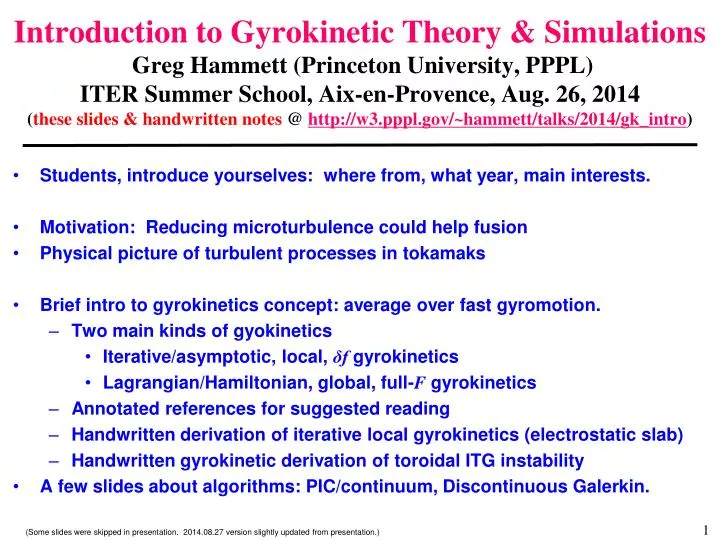
1. Introduction to Gyrokinetic Theory & Simulations Greg Hammett (Princeton University, PPPL)ITER Summer School, Aix-en-Provence, Aug. 26, 2014(these slides & handwritten notes @ http://w3.pppl.gov/~hammett/talks/2014/gk_intro) • Students, introduce yourselves: where from, what year, main interests. • Motivation: Reducing microturbulence could help fusion • Physical picture of turbulent processes in tokamaks • Brief intro to gyrokinetics concept: average over fast gyromotion. • Two main kinds of gyokinetics • Iterative/asymptotic, local, δfgyrokinetics • Lagrangian/Hamiltonian, global, full-Fgyrokinetics • Annotated references for suggested reading • Handwritten derivation of iterative local gyrokinetics(electrostatic slab) • Handwritten gyrokinetic derivation of toroidal ITG instability • A few slides about algorithms: PIC/continuum, Discontinuous Galerkin. (Some slides were skipped in presentation. 2014.08.27 version slightly updated from presentation.)

2. Candy, Waltz (General Atomics) Gyrokinetic Simulation of Tokamak Microturbulence

3. Improving Confinement Can Significantly ↓ Size & Construction Cost of Fusion Reactor Well known that improving confinement & β can lower Cost of Electricity / kWh, at fixed power output. Even stronger effect if consider smaller power: better confinement allows significantly smaller size/cost at same fusion gain Q (nTτE). Standard H-mode empirical scaling: τE ~ H Ip0.93 P-0.69 B0.15 R1.97 … (P = 3VnT/τE & assume fixed nTτE, q95, βN, n/nGreenwald): R ~ 1 / ( H2.4 B1.7 ) ITER stdH=1, steady-state H~1.5 ARIES-AT H~1.5 MIT ARC (fire.pppl.gov FESAC) H89/2 ~ 1.4 (new HTS ~Bx2, Pfus ~ B4at fixed ) Relative Construction Cost n ~ const. n ∝ nGreenwald (Plots assumes a/R=0.25, cost ∝R2 roughly. Plot accounts for constraint on B @ magnet with 1.16 m blanket/shield, i.e. B = Bmag (R-a-aBS)/R) 3

4. Interesting Ideas To Improve Fusion * Liquid metal (lithium, tin) films or flows on walls: (1) protects solid wall (2) absorbs incident hydrogen ions, reduces recycling of cold neutrals back to plasma, raises edge temperature & improves global performance. TFTR found: ~2 keV edge temperature. NSTX, LTX: more lithium is better, where is the limit? * Spherical Tokamaks (STs) appear to be able to suppress much of the ion turbulence: PPPL & Culham upgrading 1 --> 2 MA to test scaling * Advanced tokamaks, alternative operating regimes (reverse magnetic shear or “hybrid”), methods to control Edge Localized Modes, higher plasma shaping. Will beam-driven or spontaneous rotation be more important than previously thought? * Tokamaks spontaneously spin: can reduce turbulence and improve MHD stability. Can we enhance this with up-down-asymmetric tokamaks or non-stellarator-symmetric stellarators with quasi-axisymmetry? * Many possible stellarator designs, room for further optimization: Quasi-symmetry / quasi-isodynamic improvements discovered relatively recently, after 40 years of fusion research. Stellarators fix disruptions, steady-state, density limit. * Robotic manufacturing advances: reduce cost of complex, precision, specialty items

5. Intuitive picture of tokamak instabilities-- based on analogy with Inverted Pendulum / Rayleigh-Taylor instability: -- curved magnetic field lines  effective gravity

6. Unstable Inverted Pendulum g L Stable Pendulum L M F=Mg ω=(g/L)1/2 (rigid rod) ω= (-g/|L|)1/2 = i(g/|L|)1/2 = iγ Instability Inverted-density fluid ⇒Rayleigh-Taylor Instability Density-stratified Fluid ρ=exp(-y/L) ρ=exp(y/L) stableω=(g/L)1/2 Max growth rateγ=(g/L)1/2

7. “Bad Curvature” instability in plasmas ≈ Inverted Pendulum / Rayleigh-Taylor Instability Growth rate: Top view of toroidal plasma: Similar instability mechanism in MHD & drift/microinstabilities 1/L = |∇p|/p in MHD, ∝ combination of ∇n & ∇T in microinstabilities. R plasma = heavy fluid B = “light fluid” geff = centrifugal force

8. The Secret for Stabilizing Bad-Curvature Instabilities Twist in B carries plasma from bad curvature region to good curvature region: Unstable Stable Similar to how twirling a honey dipper can prevent honey from dripping.

10. An aside to define some tokamak terminology (𝜄 used in stellarator literature): q ≈1.6 in the upper right figure 2 slides back.

12. Spherical Torus has improved confinement and pressure limits (but less room in center for coils) ST max beta ~ 100% (locally, smaller relative to field at coil) Tokamak max beta ~ 10%

13. These physical mechanisms can be seen in gyrokinetic simulations and movies Unstable bad-curvature side, eddies point out, direction of effective gravity Stable side, smaller eddies particles quickly move along field lines, so density perturbations are very extended along field lines, which twist to connect unstable to stable side

15. Note: previous and other figures show color contours of density fluctuations, not of the total density, because if one plotted contours of total density, the tiny fluctuations would not be visible: For low-frequency fluctuations, ω << k|| vte, electrons have a Boltzmann response to lowest order along a field line: So contours of density fluctuations are also contours of constant potential, and so represent stream lines for the ExB drift. (Like stream lines in 2D fluid flow.) Can illustrate this with a sketch…

16. Moviehttps://fusion.gat.com/theory-wiki/images/3/35/D3d.n16.2x_0.6_fly.mpg from http://fusion.gat.com/theory/Gyromovies shows contour plots of density fluctuations in a cut-away view of a GYRO simulation (Candy & Waltz, GA). This movie illustrates the physical mechanisms described in the last few slides. It also illustrates the important effect of sheared flows in breaking up and limiting the turbulent eddies. Long-wavelength equilibrium sheared flows in this case are driven primarily by external toroidal beam injection. (The movie is made in the frame of reference rotating with the plasma in the middle of the simulation. Barber pole effect makes the dominantly-toroidal rotation appear poloidal..) Short-wavelength, turbulent-driven flows also play important role in nonlinear saturation. Sheared flows More on sheared-flow suppression of turbulence later

17. Sheared flows can suppress or reduce turbulence Most Dangerous Eddies: Transport long distances In bad curvature direction Sheared Eddies Less effective Eventually break up = + Sheared Flows Biglari, Diamond, Terry (Phys. Fluids1990), Carreras, Waltz, Hahm, Kolmogorov, et al.

18. Sheared ExB Flows can regulate or completely suppress turbulence (analogous to twisting honey on a fork) Dominant nonlinear interaction between turbulent eddies and ±θ-directed zonal flows. Additional large scale sheared zonal flow (driven by beams, neoclassical) can completely suppress turbulence Waltz, Kerbel, Phys. Plasmas 1994 w/ Hammett, Beer, Dorland, Waltz Gyrofluid Eqs., Numerical Tokamak Project, DoE Computational Grand Challenge

19. Simple picture of reducing turbulence by negative magnetic shear Particles that produce an eddy tend to follow field lines. Reversed magnetic shear twists eddy in a short distance to point in the ``good curvature direction''. Locally reversed magnetic shear naturally produced by squeezing magnetic fields at high plasma pressure: ``Second stability'' Advanced Tokamak or Spherical Torus. Shaping the plasma (elongation and triangularity) can also change local shear (in std tokamaks) Advanced Tokamaks Fig. from Antonsen, Drake, Guzdar et al. Phys. Plasmas 96 Kessel, Manickam, Rewoldt, Tang Phys. Rev. Lett. 94 “Normal” in stellarators

20. R. Nazikian et al.

21. R. Nazikian et al.

23. All major tokamaks show turbulence can be suppressed w/ sheared flows & negative magnetic shear / Shafranov shift Synakowski, Batha, Beer, et.al. Phys. Plasmas 1997 Internal transport barrier forms when the flow shearing rate dvθ /dr > ~ the max linear growth rate γlinmax of the instabilities that usually drive the turbulence. Shafranov shift Δ’ effects (self-induced negative magnetic shear at high plasma pressure) also help reduce the linear growth rate. Advanced Tokamak goal: Plasma pressure ~ x 2, Pfusion∝ pressure2 ~ x 4

24. Turbulence suppression mechanisms really work:Ion Transport level can be reduced to minimal collisional level in some cases.

27. Rosenbluth-Longmire picture

28. Can repeat this analysis on the good curvature side & find it is stable. (Leave as exercise.) Rosenbluth-Longmire picture

29. Rigorous derivation of ITG growth rate & threshold (in a simple limit) starting from the Gyrokinetic Eq. (see handwritten notes…)

30. Fairly Comprehensive 5-D Gyrokinetic Turbulence Codes Have Been Developed small scale, small amplitude density fluctuations (<1%) suppressed by reversed magnetic shear • Solve for the particle distribution function f(r,θ,α,E,μ,t) (avg. over gyration: 6D  5D) • 500 radii x 32 complex toroidal modes (96 binormal grid points) x 10 parallel points along half-orbitsx 8 energies x 16 v||/v12 hours on ORNL Cray X1E w/ 256 MSPs • Realistic toroidal geometry, kinetic ions & electrons, finite-β electro-magnetic fluctuations, full linearized collisions. • Sophisticated spectral/high-order upwind algorithms. This plot from continuum/Eulieran code GYRO (SciDAC project), GENE (Garching) similar. These and other codes being widely compared with experiments. (Candy, Waltz, General Atomics)

31. Major breakthrough: Gyrokinetic predictions now much better than 1990 analytic turbulence theories JET L-mode 19649 meas. sim. χi(cm2/s) Measured Gyrokinetic simulations agree fairly well with most experiments. Demonstrates feasibility of directly coupling gyrokinetic turbulence codes to long-time-scale transport codes. r (cm) Plot made in 1990. Analytic theories disagreed with measured diffusion coefficients by factors of 100-1000. The importance of thresholds for marginal stability not appreciated then. Explains why the edge effects the core so much.(see also S.D. Scott et al., Phys. Fluids B 1990) Barnes, Dorland, et al., PoP 2010

32. Gyro-Bohm Mixing-length estimate of diffusion caused by microturbulence eddies: Peaks at r ~ 0 where T is high. Contradicts expts. More generally, there is usually a threshold for the instability: (IFS-PPPL transport model, Kotschenreuther, Dorland, Beer, Hammett, Phys. Plasmas 1995, also GLF23, TGLF, and other models) Small where T is high, explains χ(r) decreasing near axis in expts.

33. Heat Flux Hot Core Cool Edge

34. Heat Flux Hot Core Cool Edge

35. Heat Flux Hot Core Cool Edge In hot core, no matter how much heating power , you just get (approx.) marginal stability: ⇒ C set by boundary conditions near edge where marginal stability breaks down.

36. Sheldon uses gyrokinetic theory to design a fusion reactor TV sitcom “The Big Bang Theory”, Jan. 31, 2013 "The Cooper/Kripke Inversion”. Equation for critical-gradient plasma turbulence from gyrokinetic/gyrofluid simulations based on work by Dorland, Kotschenreuther, Hammett, Beer, Waltz, Biglari et al., see slide #34 of http://w3.pppl.gov/~hammett/talks/2005/kitp-fusion-status.pdf Gyrorbit picture from Krommes 2012, http://dx.doi.org/10.1146/annurev-fluid-120710-101223.

37. Gyrokinetic-based TGLF transport model compares well with core of many experiments Biggest gap: doesn’t predict edge region (r/a>0.8). Kinsey et al. Nucl. Fus. 2011 http://stacks.iop.org/NF/51/083001

38. Motivation: Need comprehensive simulations of edge, because pedestal temperature has big effect on fusion gain Q Because of marginal stability effects, the edge boundary condition strongly affects the core: the edge is the tail that wags the dog. Need an edge code to answer many important questions: height of the pedestal, conditions for H-mode transport barrier formation, effect of RMP coils to suppress ELMs, divertor power handling, improvements with lithium walls... Kinsey et al. Nucl. Fus. 2011 http://stacks.iop.org/NF/51/083001

39. Edge pedestaltemperature profile near the edge of an H-mode discharge in the DIII-D tokamak. [Porter2000]. Pedestal is shaded region. 1000 Temp. (eV) 500 0 R (cm) Edge region very difficult Present core gyrokinetic codes are highly optimized for core, need new codes to handle additional complications of edge region of tokamaks (& stellarators): open & closed field lines, plasma-wall-interactions, large amplitude fluctuations, positivity constraints, atomic physics, non-axisymmetric RMP / stellarator coils, magnetic fluctuations near beta limit… Hard problem: but success of core gyrokinetic codes makes me believe this is tractable, with a major initiative

40. if low frequencies ω << cyclotron frequency (Ωc),  average over particle gyration, treat particles as rings of charge in spatially varying fields • Development of & physics in gyrokinetic equations When calculating charge at point Q, have to sum over all particles whose guiding centers are on the dashed line, & have to include small variation of particle density around gyro-orbit ( polarization shielding) Development of nonlinear gyrokinetics was a major breakthrough potential averaged around particle orbit, even if k⊥ρi large Based on B.D. Scott

41. Development of & physics in Gyrokinetic Eqs. Development of gyrokinetic equations one of the triumphs of high-power theoretical plasma physics and applied math (asymptotic analysis) Interesting pre-history and history of gyrokinetics… Key advance: Frieman & Chen (79-82) show nonlinear gyrokinetics possible, used an iterative local approach Another version of gyrokinetics: Hamiltonian / Lagrangian Field-Theory derivations (Hahm, Brizard, Qin, Sugama, …), insuresconservation properties for global codes, easier to go to higher order

42. Deriviation of MHD-Drift-Kinetic Eq.: * R. M. Kulsrud, in Proc. International School of Physics Enrico Fermi, Course XXV, Advanced Plasma Theory, edited by M. N. Rosenbluth, Varenna, Italy, 1962. * R. M. Kulsrud, in Handbook of Plasma Physics, edited by M. N. Rosenbluth & R. Z. Sagdeev, 1983.

43. Big Breakthrough: Nonlinear Gyrokinetics • Long, interesting history of linear gyrokinetics, 1960’s, 1970’s. • E. A. Frieman & L. Chen 79-82, showed it is possible to gyro-average nonlinear terms and keep full FLR-effects for arbitrary k⊥ρ, & get rigorous solution w/o closure problem. Very impressive. Triumph of asymptotic analysis and theoretical insight. • (usually, averaging nonlinear terms  closure problems, such as fluid equation closures, statistical turbulence theories,...Perhaps some understood, or in retrospect: J.B. Taylor ’67 showed adiabatic invariant still exists at arbitrary k⊥ρ, for small amplitude perturbations…) • GK ordering allows capture of drift/micro-instabilities & much of MHD at just order ε & not ε2 Guided by expts., μwave scattering, physics insights

45. (written in slightly different way in Lagrangian forms of gyrokinetics to get exact energy and phase-space conservation for global codes.)

47. (borrowed from B. D. Scott)

48. Polarization Density Plays Key Role in Gyrokinetic Poisson / QuasineutralityEq. At long wavelengths (neglecting higher-order FLR corrections to polarization density): Looks like a Poisson equation, but actually is a statement of quasineutrality: -(Polarization charge density) = guiding center charge density (including gyroaveraging) Because the polarization density depends on the potential, this is how the potential gets determined. The polarization density can be shown to be related to the higher-order polarization drift:

49. Polarization Density Plays Key Role in Gyrokinetic Poisson / QuasineutralityEq. At long wavelengths (neglecting higher-order FLR corrections to polarization density): In order for a non-local/global gyrokinetic code to have a conservedenergy-like quantity using just the lowest order drifts (ExB, grad(B) and curvature) from the first order Hamiltonian H1 ~ (ρ/L) T, the density on the LHS must be replaced by a time-independent ns0. In order to allow a time varying ns, and conserve the energy properly, one must include drifts from the second order Hamiltonian H2~ (ρ/L)2 T. Natural consequence of Lagrangian field theory approach. • (Local gyrokinetics also satisfies energy conservation, H2 effectsincorporated in the higher-order transport equations.)

50. alternative derivation: next order correction to adiabatic invariant mu