Download
1 / 32
330 likes | 380 Views
Explore the theoretical studies and experimental findings on ultrafast solvation dynamics and ionic conductivity in aqueous solutions. Discover the factors influencing solvation dynamics and ion mobility in different solvents. Learn about the role of translational modes and the impact of ion-dipole forces on conductivity.

E N D
Ionic Conductivity And Ultrafast Solvation Dynamics Biman Bagchi Indian Institute of Science Bangalore, INDIA
The values of the limiting ionic conductivity (0) of rigid, mono positive ions in water at 298 K are plotted as a function of the inverse of the crystallography ionic radius, r-1ion. Biswas and Bagchi J. Am. Chem. Soc. 119, 5946 (1997)
Ionic Conductivity What determines the conductivity of an ion in a dilute electrolyte solution ? • The forces acting on the ion can be divided into two type : Short range force and the long range ion-dipole forces. The former can be related to viscosity via Stokes relation. The long range force part is the one which is responsible for the anomalous behavior of ionic conductance. Continuum models of Hubbard-Onsagar-Zwanzig neglected the molecularity. • The theory of Calef and Wolynes treated the dipolar response as over damped, but emphasized the role oftranslational motion of the solvent molecules.
Consider the mobility of an ion in a dipolar liquid, like water or acetonitrile • The ionic mobility is determined by diffusion which in turn is determined by the friction on the ion, via Einstein relation. = SR + DF The classical theory ( Hubbard-Onsagar-Zwanzig ) finds that the friction on the ion, and hence the mobility, depends inversely on the Debye relaxation time D , which is the slowest time. This leads to the well-known law of Walden’s product which states that the product of the limiting ionic conductivity (0) of an electrolyte and the viscosity () is inversely proportional to the radius (rion) of the ion.
Ultrafast solvation and ionic mobility Two kinds of friction : Stokes friction (0) and Dielectric friction (DF) How to getDF ? What determines DF ?
All the earlier theoretical studies ignored the ultrafast response of the dipolar solvents. (Zwanzig, Hubbard-Wolynes, Felderhof ….) Theory however shows that they are important, in two ways. First, they are reduce the friction on the ion by allowing the relaxation of the force on the ion. Second, they make the role of the translational modes less important. What is even more important is the relative role of various ultrafast components.
Lots have been found about solvation dynamics of ions in water. Potential Energy Surfaces involved in Solvation Dynamics Water orientational motions along the solvation coordinate together with instantaneous polarization P Pal, Peon, Bagchi and Zweail J. Phys. Chem. Phys. B 106, 12376 (2002)
Continuum Model of Solvation Dynamics [BFO (1984), vdZH (1985)]
Polarization relaxation is single exponential. Debye representation For ion For water, L 500 fs
Ultrafast solvation dynamics in water, Acetonitrile and Methanol • However, initial solvation dynamics in water and acetonitrile was found to be much faster. For water it is found to be less than 50 fs!! • In addition, the ultrafast component carried about 60-70% of the total relaxation strength. • Such an ultrafast component can play significant role in many chemical processes in water.
Experimental (‘expt’; s(t)) and simulated (‘q’; c(t)) solvation response function for c343 in water. Also shown is a simulation for a neutral atomic solute with the Lennard-Jones parameters of the water oxygen atom (S0). R. Jlmenez et al. Nature 369, 471 (1994)
Theoretical Approach Nandi, Roy and Bagchi, J. Chem. Phy. 102, 1390 (1995); Song, Marcus & Chandler, JCP (2000).
Mode coupling theory expression for solvation time correlation function Where AN is the normalization constant cid(k) and Ssolv(k,t) are the ion-dipole DCF and the orientational dynamic structure factor of the pure solvent. Sion(k,t) denotes the self-dynamics structure factor of the ion.
The rate of the decay of the orientational dynamics solvent factor, S10solv(k,t/) as a function of time (t), for water at two different temperature (solid line-318K, dashed line-283K). Note that the numerical results obtained with k = 2 and = 1× 10-12 s.
Microscopic origin of Ultrafast solvation k 0 k 2/ In the bulk, the k component dominates (about 75 %). However, this is only part of the story. Dynamics response comes into picture. 0
Effect of translational modes on ionic conductivity and solvation dynamics.
MCT Expression for Dielectric Friction including the self-motion » N-E equation » S-E equation The position dependent viscosity is given by
Where,
Experimental values of the Walden product (00 ) of rigid , monopositive ions in water (open triangle), acetonitrile and fomamide (open squares) at 298 K are plotted as a function of the inverse of the crystallography ionic radius (r-1ion). Bagchi and Biswas Adv. Chem. Phys. 109, 207 (1999)
The values of the limiting ionic conductivity (0) of rigid, mono positive ions in water at 298 K are plotted as a function of the inverse of the crystallography ionic radius, r-1ion.
The inverse of the calculated stokes radius (rstokes) is plotted against the respective crystallographic radius (rion) in acetonitrile and water respectively. Biswas, Roy and Bagchi, Phys. Rev. Lett. 75, 1098 (1995)
The effect of the sequential addition of the ultrafast component of the solvent orientational motion on the limiting ionic in methanol at 298 K. The curves labeled 1, 2 and 3 are the predictions of the present molecular theory.
The effect of isotopic substitution on limiting ionic conductivity in electrolyte solution.
Concentration dependence of ionic self-diffusion J. –F. Dufreche et al. PRL 88, 95902 (2002).
Velocity correlation function of Cl- for c = 0.5M and c = 1M KCl solutions. Comparison between MCT (solid line) and Brownian dynamics (dashed line).
Time dependent self-diffusion coefficient of Cl-for c = 0.5M and c = 1M KCl solutions. Comparison between MCT (solid line) and Brownian dynamics (dashed line).
Mode coupling theory of ionic conductivity The total conductance of aqueous (a) KCl (b) NaCl solution is plotted against the square root of ion concentration. The solid curve represents the prediction of the theory and the square represents the experimental results. Chandra and Bagchi J. Phys. Chem. B 104, 9067 (2000)
Mode coupling theory of ionic viscosity The ionic contribution to the viscosity is plotted against the square root of ion concentration (in molarity) for solutions of (a) 1:1 and (b) 2:2 electrolytes. The reduced viscosity .
Acknowledgement • Prof. Srabani Roy, IIT-Kharagpur • Prof. Nilashis Nandi, BITS-Pilanyi • Prof. A. Chandra, IIT-Kanpur • DST, CSIR
The prediction from dynamic mean spherical approximation (DMSA) for solvation time correlation function and the comparison between the ionic and the dipolar solvation dynamics. Nandi, Roy and Bagchi, J. Chem. Phy. 102, 1390 (1995)
The ratio of the microscopic polarization to the macroscopic polarization is plotted as a function of r for water at 298K.