Download
1 / 60
610 likes | 755 Views
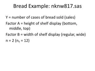
Bread Example: nknw817.sas. Y = number of cases of bread sold (sales) Factor A = height of shelf display (bottom, middle, top) Factor B = width of shelf display (regular, wide) n = 2 ( n T = 12). Bread Example: input. data bread; infile 'I:My DocumentsStat 512CH19TA07.DAT' ;

E N D
Bread Example: nknw817.sas Y = number of cases of bread sold (sales) Factor A = height of shelf display (bottom, middle, top) Factor B = width of shelf display (regular, wide) n = 2 (nT = 12)
Bread Example: input data bread; infile'I:\My Documents\Stat 512\CH19TA07.DAT'; input sales height width; procprintdata=bread; run; title1h=3'Bread Sales'; axis1label=(h=2); axis2label=(h=2angle=90);
Bread Example: input scatterplot data bread; set bread; if height eq1 and width eq1then hw='1_BR'; if height eq1 and width eq2then hw='2_BW'; if height eq2 and width eq1then hw='3_MR'; if height eq2 and width eq2then hw='4_MW'; if height eq3 and width eq1then hw='5_TR'; if height eq3 and width eq2then hw='6_TW'; title2h=2'Sales vs. treatment'; symbol1v=circle i=nonec=blue; procgplotdata=bread; plot sales*hw/haxis=axis1 vaxis=axis2; run;
Bread Example: ANOVA procglmdata=bread; class height width; model sales=height width height*width; means height width height*width; outputout=diag r=resid p=pred; run;
Bread Example: Means procmeansdata=bread; var sales; by height width; outputout=avbreadmean=avsales; procprintdata=avbread; run;
Bread Example: diagnostics procglmdata=bread; class height width; model sales=height width height*width; means height width height*width; outputout=diag r=resid p=pred run; title2h=2'residual plots'; procgplotdata=diag; plotresid * (pred height width)/vref=0 haxis=axis1 vaxis=axis2; run; title2'normality'; procunivariatedata=diagnoprint; histogramresid/normalkernel; qqplotresid/normal (mu=estsigma=est); run;
Bread Example: nknw817.sas Y = number of cases of bread sold (sales) Factor A = height of shelf display (bottom, middle, top) Factor B = width of shelf display (regular, wide) n = 2 (nT = 12) Questions: • Does the height of the display affect sales? • Does the width of the display affect sales? • Does the effect on height on sales depend on width? • Does the effect of the width depend on height?
Bread Example: Interaction Plots title2'Interaction Plot'; symbol1v=square i=join c=black; symbol2v=diamond i=join c=red; symbol3v=circle i=join c=blue; procgplotdata=avbread; plotavsales*height=width/haxis=axis1 vaxis=axis2; plotavsales*width=height/haxis=axis1 vaxis=axis2; run;
Bread Example: ANOVA table procglmdata=bread; class height width; model sales=height width height*width; means height width height*width; outputout=diag r=resid p=pred; run;
Bread Example: cell means model (MSE) procglmdata=bread; class height width; model sales=height width height*width; means height width height*width; outputout=diag r=resid p=pred; run;
Bread Example: cell means model procglmdata=bread; class height width; model sales=height width height*width; means height width height*width; outputout=diag r=resid p=pred; run;
Bread Example: factor effects model (overall mean) (cont) procglmdata=bread; class height width; model sales=; outputout=pmu p=muhat; procprintdata=pmu;run;
Bread Example: means A (cont) procglmdata=bread; class height width; model sales=height; outputout=pA p=Amean; procprintdata = pA; run;
Bread Example: Factor Effects Model (zero-sum constraints) title2'overall mean'; procglmdata=bread; class height width; model sales=; outputout=pmu p=muhat; procprintdata=pmu; run; title2 'mean for height'; procglmdata=bread; class height width; model sales=height; outputout=pA p=Amean; procprintdata = pA; run; title2'mean for width'; procglmdata=bread; class height width; model sales=width; outputout=pB p=Bmean; run; title2'mean height/ width'; procglmdata=bread; class height width; model sales=height*width; outputout=pAB p=ABmean; run; dataparmest; merge bread pmupApBpAB; alpha=Amean-muhat; beta=Bmean-muhat; alphabeta=ABmean-(muhat+alpha+beta); run; procprint;run;
Bread Example: Factor Effects Model (zero-sum constraints) (cont)
Bread Example: nknw817b.sas Y = number of cases of bread sold (sales) Factor A = height of shelf display (bottom, middle, top) Factor B = width of shelf display (regular, wide) n = 2 (nT = 12 = 3 x 2)
Bread Example: SAS constraints procglmdata=bread; class height width; model sales=height width height*width/solution; means height*width; run;
Bread Example: nknw817b.sas Y = number of cases of bread sold (sales) Factor A = height of shelf display (bottom, middle, top) Factor B = width of shelf display (regular, wide) n = 2 (nT = 12 = 3 x 2)
Bread Example: Pooling *factor effects model, SAS constraints, without pooling; procglmdata=bread; class height width; model sales=height width height*width; means height/tukeylines; run; *with pooling; procglmdata=bread; class height width; model sales=height width; means height / tukeylines; run;
Bread Example (nknw864.sas): contrasts and estimates procglmdata=bread; class height width; model sales=height width height*width; contrast'middle vs others' height -.51 -.5 height*width -.25 -.25.5.5 -.25 -.25; estimate'middle vs others' height -.51 -.5 height*width -.25 -.25.5.5 -.25 -.25; means height*width; run;
Car Insurance Example: (nknw878.sas) Y = 3-month premium for car insurance Factor A = size of the city small, medium, large Factor B = geographic region east, west
Car Insurance: input datacarins; infile'I:\My Documents\Stat 512\CH20TA02.DAT'; input premium size region; if size=1thensizea='1_small '; if size=2thensizea='2_medium'; if size=3thensizea='3_large '; procprintdata=carins; run;
Car Insurance: Scatterplot symbol1v='E'i=join c=green height=1.5; symbol2v='W'i=join c=blue height=1.5; title1h=3'Scatterplot of the Car Insurance'; procgplotdata=carins; plot premium*sizea=region/haxis=axis1 vaxis=axis2; run;
Car Insurance: ANOVA procglmdata=carins; classsizea region; model premium=sizea region/solution; meanssizea region / tukey; outputout=preds p=muhat; run; procprintdata=preds; run;