Download
1 / 41
410 likes | 529 Views
On-Shell Methods in Gauge Theory. David A. Kosower IPhT, CEA–Saclay Taiwan Summer Institute, Chi-Tou (溪頭) August 10–17, 2008 Lecture I. Tools for Computing Amplitudes. New tools for computing in gauge theories — the core of the Standard Model (useful for gravity too)

E N D
On-Shell Methods in Gauge Theory David A. Kosower IPhT, CEA–Saclay Taiwan Summer Institute, Chi-Tou (溪頭) August 10–17, 2008 Lecture I
Tools for Computing Amplitudes • New tools for computing in gauge theories — the core of the Standard Model(useful for gravity too) • Motivations and connections • Particle physics: SU(3) SU(2) U(1) • N =4 supersymmetric gauge theories and AdS/CFT • Witten’s twistor string
On-Shell Methods • Physical states • Use of properties of amplitudes as calculational tools • Kinematics: Spinor Helicity Basis Twistor space • Tree Amplitudes: On-shell Recursion Relations Factorization • Loop Amplitudes: Unitarity (SUSY) Unitarity + On-shell Recursion QCD
Outline • Review: motivations; jets; QCD and parton model; radiative corrections; • Color decomposition and color ordering; spinor product and spinor helicity • Factorization, collinear and soft limits • On-shell and off-shell recursion relations • Unitarity method and one-loop amplitudes • Loop-level on-shell recursion relations and the bootstrap • Numerical approaches • Higher loops and applications to N = 4 SUSY
Particle Physics The LHC is coming, the LHC is coming! • Why do we compute in field theory? • Why do we do hard computations? • What quantities should we compute in field theory? Within one month!
SU(3) SU(2) U(1) Standard Model • Known physics, and background to new physics • Hunting for new physics beyond the Standard Model • Discovery of new physics • Compare measurements to predictions — need to calculate signals • Expect to confront backgrounds • Backgrounds are large
Hunting for New Physics • Yesterday’s new physics is tomorrow’s background • To measure new physics, need to understand backgrounds in detail • Heavy particles decaying into SM or invisible states • Often high-multiplicity events • Low multiplicity signals overwhelmed by SM: Higgs → → 2 jets • Predicting backgrounds requires precision calculations of known Standard Model physics
Complexity is due to QCD • Perturbative QCD: Gluons & quarks → gluons & quarks • Real world: Hadrons → hadrons with hard physics described by pQCD • Hadrons → jets narrow nearly collimated streams of hadrons
Jets • Defined by an experimental resolution parameter • invariant mass in e+e− • cone algorithm in hadron colliders: cone size in and minimum ET • kT algorithm: essentially by a relative transverse momentum CDF (Lefevre 2004)1374 GeV
In theory, theory and practice are the same. In practice, they are different — Yogi Berra
The Challenge • Everything at a hadron collider (signals, backgrounds, luminosity measurement) involves QCD • Strong coupling is not small: s(MZ) 0.12 and running is important • events have high multiplicity of hard clusters (jets) • each jet has a high multiplicity of hadrons • higher-order perturbative corrections are important • Processes can involve multiple scales: pT(W) & MW • need resummation of logarithms • Confinement introduces further issues of mapping partons to hadrons, but for suitably-averaged quantities (infrared-safe) avoiding small E scales, this is not a problem (power corrections)
CDF, PRD 77:011108 Leading-Order, Next-to-Leading Order • LO: Basic shapes of distributionsbut: no quantitative prediction — large scale dependence missing sensitivity to jet structure & energy flow • NLO: First quantitative prediction improved scale dependence — inclusion of virtual corrections basic approximation to jet structure — jet = 2 partons • NNLO: Precision predictions small scale dependence better correspondence to experimental jet algorithms understanding of theoretical uncertainties Anastasiou, Dixon, Melnikov, & Petriello
What Contributions Do We Need? • Short-distance matrix elements to 2-jet production at leading order: tree level
Short-distance matrix elements to 2-jet production at next-to-leading order: tree level + one loop + real emission 2
Real-Emission Singularities Matrix element Integrate
Physical quantities are finite • Depend on resolution parameter • Finiteness thanks to combination of Kinoshita–Lee–Nauenberg theorem and factorization • Singularities in virtual corrections canceled by those in real emission
Tree Amplitudes • First step in any physics process — leading-order contribution • But also — the key ingredient in loop calculations
Traditional Tool: Feynman Diagrams • Write down all Feynman diagrams for the desired process • Write out all vertex factors, kinematic and color, and contract indices with propagators • Square amplitude, contracting polarization vectors or fermion wavefunctions by summing over helicities • Yields expressions in terms of momentum invariants • But unmanageably large ones
So What’s Wrong with Feynman Diagrams? • Huge number of diagrams in calculations of interest — factorial growth • 2 → 6 jets: 34300 tree diagrams, ~ 2.5 ∙ 107 terms ~2.9 ∙ 106 1-loop diagrams, ~ 1.9 ∙ 1010 terms • But answers often turn out to be very simple • Vertices and propagators involve gauge-variant off-shell states • Each diagram is not gauge invariant — huge cancellations of gauge-noninvariant, redundant, parts in the sum over diagrams Simple results should have a simple derivation — attr to Feynman • Want approach in terms of physical states only
Light-Cone Gauge Only physical (transverse) degrees of freedom propagate physical projector — two degrees of freedom
Color Decomposition Standard Feynman rules function of momenta, polarization vectors , and color indices Color structure is predictable. Use representation to represent each term as a product of traces, and the Fierz identity
To unwind traces Leads to tree-level representation in terms of single traces Color-ordered amplitude — function of momenta & polarizations alone; not Bose symmetric
Symmetry properties • Cyclic symmetry • Reflection identity • Parity flips helicities • Decoupling equation
Amplitudes Functions of momenta k, polarization vectors for gluons; momenta k, spinor wavefunctions ufor fermions Gauge invariance implies this is a redundant representation: k: A = 0
Spinor Variables From Lorentz vectors to bi-spinors 2×2 complex matrices with det = 1 ‘Chinese Magic’ Xu, Zhang, Chang (1984) Spinor-helicity basis
We have explicit formulæ otherwise so that the identity always holds Properties Transverse Normalized
Properties of the Spinor Product • Antisymmetry • Gordon identity • Charge conjugation • Fierz identity • Projector representation • Schouten identity
Color decomposition & stripping Gauge-theory amplitude Color-ordered amplitude: function of kiand i Helicity amplitude: function of spinor variables and helicities ±1 Spinor-helicity basis
Calculate choose identical reference momenta for all legs all vanish amplitude vanishes Calculate choose reference momenta 4,1,1,1 all vanish amplitude vanishes Calculate choose reference momenta 3,3,2,2 only nonvanishing is (*,2,3) vertex vanishes only s12 channel contributes
No diagrammatic calculation required for the last helicity amplitude, Obtain it from the decoupling identity
These forms hold more generally, for larger numbers of external legs: Parke-Taylor equations Mangano, Xu, Parke (1986) Maximally helicity-violating or ‘MHV’ Proven using the Berends–Giele recurrence relations Berends & Giele (1988)
J5 appearing inside J10 is identical to J5 appearing inside J17 • Imagine computing all subcurrents ‘bottom up’: first compute J3, then J4 , and so on. • O(n) different color-ordered currents Jk for each k appearing in n-point amplitude, n different ks • Compute once numerically maximal reuse • Computing each takes O(n2) steps (because of the four-point vertex) • Polynomial complexity per helicity: O(n4)