Download
1 / 92
930 likes | 1.09k Views
PETSc Tutorial. Numerical Software Libraries for the Scalable Solution of PDEs. Satish Balay, Kris Buschelman, Bill Gropp, Dinesh Kaushik, Matt Knepley, Lois Curfman McInnes, Barry Smith, Hong Zhang Mathematics and Computer Science Division Argonne National Laboratory

E N D
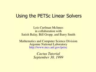
PETSc Tutorial Numerical Software Libraries for the Scalable Solution of PDEs Satish Balay, Kris Buschelman, Bill Gropp, Dinesh Kaushik, Matt Knepley, Lois Curfman McInnes, Barry Smith, Hong Zhang Mathematics and Computer Science Division Argonne National Laboratory http://www.mcs.anl.gov/petsc Intended for use with version 2.1.0 of PETSc
The Role of PETSc • Developing parallel, non-trivial PDE solvers that deliver high performance is still difficult and requires months (or even years) of concentrated effort. • PETSc is a toolkit that can ease these difficulties and reduce the development time, but it is not a black-box PDE solver nor a silver bullet.
What is PETSc? • A freely available and supported research code • Available via http://www.mcs.anl.gov/petsc • Free for everyone, including industrial users • Hyperlinked documentation and manual pages for all routines • Many tutorial-style examples • Support via email: petsc-maint@mcs.anl.gov • Usable from Fortran 77/90, C, and C++ • Portable to any parallel system supporting MPI, including • Tightly coupled systems • Cray T3E, SGI Origin, IBM SP, HP 9000, Sun Enterprise • Loosely coupled systems, e.g., networks of workstations • Compaq, HP, IBM, SGI, Sun • PCs running Linux or Windows • PETSc history • Begun in September 1991 • Now: over 8,500 downloads since 1995 (versions 2.0 and 2.1) • PETSc funding and support • Department of Energy: MICS Program, DOE2000, SciDAC • National Science Foundation, Multidisciplinary Challenge Program, CISE
PETSc Concepts • How to specify the mathematics of the problem • Data objects • vectors, matrices • How to solve the problem • Solvers • linear, nonlinear, and time stepping (ODE) solvers • Parallel computing complications • Parallel data layout • structured and unstructured meshes
PETSc PDE Application Codes ODE Integrators Visualization Nonlinear Solvers, Unconstrained Minimization Interface Linear Solvers Preconditioners + Krylov Methods Object-Oriented Matrices, Vectors, Indices Grid Management Profiling Interface Computation and Communication Kernels MPI, MPI-IO, BLAS, LAPACK Structure of PETSc
PETSc Numerical Components Nonlinear Solvers Time Steppers Newton-based Methods Other Euler Backward Euler Pseudo Time Stepping Other Line Search Trust Region Krylov Subspace Methods GMRES CG CGS Bi-CG-STAB TFQMR Richardson Chebychev Other Preconditioners Additive Schwartz Block Jacobi Jacobi ILU ICC LU (Sequential only) Others Matrices Compressed Sparse Row (AIJ) Blocked Compressed Sparse Row (BAIJ) Block Diagonal (BDIAG) Dense Matrix-free Other Distributed Arrays Index Sets Indices Block Indices Stride Other Vectors
What is not in PETSc? • Discretizations • Unstructured mesh generation and refinement tools • Load balancing tools • Sophisticated visualization capabilities But PETSc does interface to external software that provides some of this functionality.
Flow of Control for PDE Solution Main Routine Timestepping Solvers (TS) Nonlinear Solvers (SNES) Linear Solvers (SLES) PETSc PC KSP Application Initialization Function Evaluation Jacobian Evaluation Post- Processing User code PETSc code
PETSc emphasis Levels of Abstraction in Mathematical Software • Application-specific interface • Programmer manipulates objects associated with the application • High-level mathematics interface • Programmer manipulates mathematical objects, such as PDEs and boundary conditions • Algorithmic and discrete mathematics interface • Programmer manipulates mathematical objects (sparse matrices, nonlinear equations), algorithmic objects (solvers) and discrete geometry (meshes) • Low-level computational kernels • e.g., BLAS-type operations
The PETSc Programming Model • Goals • Portable, runs everywhere • Performance • Scalable parallelism • Approach • Distributed memory, “shared-nothing” • Requires only a compiler (single node or processor) • Access to data on remote machines through MPI • Can still exploit “compiler discovered” parallelism on each node (e.g., SMP) • Hide within parallel objects the details of the communication • User orchestrates communication at a higher abstract level than message passing
Collectivity • MPI communicators (MPI_Comm) specify collectivity (processors involved in a computation) • All PETSc creation routines for solver and data objects are collective with respect to a communicator, e.g., • VecCreate(MPI_Comm comm, int m, int M, Vec *x) • Some operations are collective, while others are not, e.g., • collective:VecNorm() • not collective: VecGetLocalSize() • If a sequence of collective routines is used, they must be called in the same order on each processor.
Hello World #include “petsc.h”int main( int argc, char *argv[] ){ PetscInitialize(&argc,&argv,PETSC_NULL,PETSC_NULL); PetscPrintf(PETSC_COMM_WORLD,“Hello World\n”); PetscFinalize(); return 0;}
Data Objects • Vectors (Vec) • focus: field data arising in nonlinear PDEs • Matrices (Mat) • focus: linear operators arising in nonlinear PDEs (i.e., Jacobians) • Object creation • Object assembly • Setting options • Viewing • User-defined customizations beginner beginner intermediate intermediate advanced tutorial outline: data objects
Vectors proc 0 • What are PETSc vectors? • Fundamental objects for storing field solutions, right-hand sides, etc. • Each process locally owns a subvector of contiguously numbered global indices • Create vectors via • VecCreate(...,Vec *) • MPI_Comm - processors that share the vector • number of elements local to this processor • or total number of elements • VecSetType(Vec,VecType) • Where VecType is • VEC_SEQ, VEC_MPI, or VEC_SHARED proc 1 proc 2 proc 3 proc 4 data objects: vectors beginner
Vector Assembly • VecSetValues(Vec,…) • number of entries to insert/add • indices of entries • values to add • mode: [INSERT_VALUES,ADD_VALUES] • VecAssemblyBegin(Vec) • VecAssemblyEnd(Vec) data objects: vectors beginner
Parallel Matrix and Vector Assembly • Processors may generate any entries in vectors and matrices • Entries need not be generated on the processor on which they ultimately will be stored • PETSc automatically moves data during the assembly process if necessary data objects: vectors and matrices beginner
Matrices • What are PETSc matrices? • Fundamental objects for storing linear operators (e.g., Jacobians) • Create matrices via • MatCreate(…,Mat *) • MPI_Comm - processors that share the matrix • number of local/global rows and columns • MatSetType(Mat,MatType) • where MatType is one of • default sparse AIJ: MPIAIJ, SEQAIJ • block sparse AIJ (for multi-component PDEs): MPIAIJ, SEQAIJ • symmetric block sparse AIJ: MPISBAIJ, SAEQSBAIJ • block diagonal: MPIBDIAG, SEQBDIAG • dense: MPIDENSE, SEQDENSE • matrix-free • etc. data objects: matrices beginner
Matrix Assembly • MatSetValues(Mat,…) • number of rows to insert/add • indices of rows and columns • number of columns to insert/add • values to add • mode: [INSERT_VALUES,ADD_VALUES] • MatAssemblyBegin(Mat) • MatAssemblyEnd(Mat) data objects: matrices beginner
Parallel Matrix Distribution • Each process locally owns a submatrix of contiguously numbered global rows. MatGetOwnershipRange(Mat A, int *rstart, int *rend) • rstart: first locally owned row of global matrix • rend -1: last locally owned row of global matrix proc 0 proc 1 proc 2 } proc 3 proc 3: locally owned rows proc 4 data objects: matrices beginner
Viewers • Printing information about solver and data objects • Visualization of field and matrix data • Binary output of vector and matrix data beginner beginner intermediate tutorial outline: viewers
Viewer Concepts • Information about PETSc objects • runtime choices for solvers, nonzero info for matrices, etc. • Data for later use in restarts or external tools • vector fields, matrix contents • various formats (ASCII, binary) • Visualization • simple x-window graphics • vector fields • matrix sparsity structure beginner viewers
Viewing Vector Fields Solution components, using runtime option -snes_vecmonitor • VecView(Vec x,PetscViewer v); • Default viewers • ASCII (sequential): PETSC_VIEWER_STDOUT_SELF • ASCII (parallel): PETSC_VIEWER_STDOUT_WORLD • X-windows: PETSC_VIEWER_DRAW_WORLD • Default ASCII formats • PETSC_VIEWER_ASCII_DEFAULT • PETSC_VIEWER_ASCII_MATLAB • PETSC_VIEWER_ASCII_COMMON • PETSC_VIEWER_ASCII_INFO • etc. velocity: v velocity: u temperature: T vorticity: z beginner viewers
Viewing Matrix Data • MatView(Mat A, PetscViewer v); • Runtime options available after matrix assembly • -mat_view_info • info about matrix assembly • -mat_view_draw • sparsity structure • -mat_view • data in ASCII • etc. beginner viewers
Linear (SLES) Nonlinear (SNES) Timestepping (TS) Context variables Solver options Callback routines Customization important concepts Solvers: Usage Concepts Solver Classes Usage Concepts tutorial outline: solvers
Linear PDE Solution Main Routine PETSc Linear Solvers (SLES) Solve Ax = b PC KSP Application Initialization Evaluation of A and b Post- Processing User code PETSc code solvers:linear beginner
Linear Solvers Goal: Support the solution of linear systems, Ax=b, particularly for sparse, parallel problems arising within PDE-based models User provides: • Code to evaluate A, b solvers:linear beginner
Sample Linear Application:Exterior Helmholtz Problem Solution Components Real Imaginary Collaborators: H. M. Atassi, D. E. Keyes, L. C. McInnes, R. Susan-Resiga solvers:linear beginner
Natural ordering Nested dissection ordering Close-up Helmholtz: The Linear System • Logically regular grid, parallelized with DAs • Finite element discretization (bilinear quads) • Nonreflecting exterior BC (via DtN map) • Matrix sparsity structure (option: -mat_view_draw) solvers:linear beginner
Linear Solvers (SLES) SLES: Scalable Linear Equations Solvers • Application code interface • Choosing the solver • Setting algorithmic options • Viewing the solver • Determining and monitoring convergence • Providing a different preconditioner matrix • Matrix-free solvers • User-defined customizations beginner beginner beginner beginner intermediate intermediate advanced tutorial outline: solvers: linear advanced
Context Variables • Are the key to solver organization • Contain the complete state of an algorithm, including • parameters (e.g., convergence tolerance) • functions that run the algorithm (e.g., convergence monitoring routine) • information about the current state (e.g., iteration number) solvers:linear beginner
Creating the SLES Context • C/C++ version ierr = SLESCreate(MPI_COMM_WORLD,&sles); • Fortran version call SLESCreate(MPI_COMM_WORLD,sles,ierr) • Provides an identical user interface for all linear solvers • uniprocessor and parallel • real and complex numbers solvers:linear beginner
Conjugate Gradient GMRES CG-Squared Bi-CG-stab Transpose-free QMR etc. Block Jacobi Overlapping Additive Schwarz ICC, ILU via BlockSolve95 ILU(k), LU (sequential only) etc. Linear Solvers in PETSc 2.0 Preconditioners (PC) KrylovMethods (KSP) solvers:linear beginner
Setting Solver Options within Code • SLESGetKSP(SLES sles,KSP *ksp) • KSPSetType(KSP ksp,KSPType type) • KSPSetTolerances(KSP ksp,PetscReal rtol, PetscReal atol,PetscReal dtol, int maxits) • etc.... • SLESGetPC(SLES sles,PC *pc) • PCSetType(PC pc,PCType) • PCASMSetOverlap(PC pc,int overlap) • etc.... solvers:linear beginner
Recursion: Specifying Solvers for Schwarz Preconditioner Blocks • Specify SLES solvers and options with “-sub” prefix, e.g., • Full or incomplete factorization -sub_pc_type lu -sub_pc_type ilu -sub_pc_ilu_levels <levels> • Can also use inner Krylov iterations, e.g., -sub_ksp_type gmres -sub_ksp_rtol <rtol> -sub_ksp_max_it <maxit> solvers: linear: preconditioners beginner
2 1 beginner intermediate Setting Solver Options at Runtime • -ksp_type [cg,gmres,bcgs,tfqmr,…] • -pc_type [lu,ilu,jacobi,sor,asm,…] • -ksp_max_it <max_iters> • -ksp_gmres_restart <restart> • -pc_asm_overlap <overlap> • -pc_asm_type [basic,restrict,interpolate,none] • etc ... 1 2 solvers:linear
2 1 beginner intermediate Linear Solvers: Monitoring Convergence • -ksp_monitor- Prints preconditioned residual norm • -ksp_xmonitor- Plots preconditioned residual norm • -ksp_truemonitor- Prints true residual norm || b-Ax || • -ksp_xtruemonitor- Plots true residual norm || b-Ax || • User-defined monitors, using callbacks 1 2 3 3 solvers:linear advanced
Helmholtz: Scalability 128x512 grid, wave number = 13, IBM SP GMRES(30)/Restricted Additive Schwarz 1 block per proc, 1-cell overlap, ILU(1) subdomain solver solvers:linear beginner
SLES: Review of Basic Usage • SLESCreate( ) - Create SLES context • SLESSetOperators( ) - Set linear operators • SLESSetFromOptions( ) - Set runtime solver options for [SLES,KSP,PC] • SLESSolve( ) - Run linear solver • SLESView( ) - View solver options actually used at runtime (alternative: -sles_view) • SLESDestroy( ) - Destroy solver solvers:linear beginner
Profiling and Performance Tuning Profiling: • Integrated profiling using -log_summary • User-defined events • Profiling by stages of an application beginner intermediate intermediate Performance Tuning: • Matrix optimizations • Application optimizations • Algorithmic tuning intermediate intermediate tutorial outline: profiling and performance tuning advanced
Profiling • Integrated monitoring of • time • floating-point performance • memory usage • communication • All PETSc events are logged if compiled with -DPETSC_LOG (default); can also profile application code segments • Print summary data with option: -log_summary • Print redundant information from PETSc routines: -log_info • Print the trace of the functions called: -log_trace profiling and performance tuning beginner
Nonlinear Solvers (SNES) SNES: Scalable Nonlinear Equations Solvers • Application code interface • Choosing the solver • Setting algorithmic options • Viewing the solver • Determining and monitoring convergence • Matrix-free solvers • User-defined customizations beginner beginner beginner beginner intermediate advanced advanced tutorial outline: solvers: nonlinear
Nonlinear PDE Solution Main Routine Nonlinear Solvers (SNES) Solve F(u) = 0 Linear Solvers (SLES) PETSc PC KSP Application Initialization Function Evaluation Jacobian Evaluation Post- Processing User code PETSc code solvers: nonlinear beginner
Nonlinear Solvers Goal: For problems arising from PDEs, support the general solution of F(u) = 0 User provides: • Code to evaluate F(u) • Code to evaluate Jacobian of F(u) (optional) • or use sparse finite difference approximation • or use automatic differentiation • AD support via collaboration with P. Hovland and B. Norris • Coming in next PETSc release via automated interface to ADIFOR and ADIC (see http://www.mcs.anl.gov/autodiff) solvers: nonlinear beginner
Nonlinear Solvers (SNES) • Newton-based methods, including • Line search strategies • Trust region approaches • Pseudo-transient continuation • Matrix-free variants • User can customize all phases of the solution process solvers: nonlinear beginner
Velocity-vorticity formulation Flow driven by lid and/or bouyancy Logically regular grid, parallelized with DAs Finite difference discretization source code: Solution Components velocity: v velocity: u temperature: T vorticity: z Sample Nonlinear Application:Driven Cavity Problem petsc/src/snes/examples/tutorials/ex19.c solvers: nonlinear Application code author: D. E. Keyes beginner
Finite Difference Jacobian Computations • Compute and explicitly store Jacobian via 1st-order FD • Dense: -snes_fd, SNESDefaultComputeJacobian() • Sparse via colorings: MatFDColoringCreate(), SNESDefaultComputeJacobianColor() • Matrix-free Newton-Krylov via 1st-order FD, no preconditioning unless specifically set by user • -snes_mf • Matrix-free Newton-Krylov via 1st-order FD, user-defined preconditioning matrix • -snes_mf_operator solvers: nonlinear beginner
2 1 beginner intermediate Uniform access to all linear and nonlinear solvers • -ksp_type [cg,gmres,bcgs,tfqmr,…] • -pc_type [lu,ilu,jacobi,sor,asm,…] • -snes_type [ls,tr,…] • -snes_line_search <line search method> • -sles_ls <parameters> • -snes_convergence <tolerance> • etc... 1 2 solvers: nonlinear
SNES: Review of Basic Usage • SNESCreate( ) - Create SNES context • SNESSetFunction( ) - Set function eval. routine • SNESSetJacobian( ) - Set Jacobian eval. routine • SNESSetFromOptions( ) - Set runtime solver options for [SNES,SLES,KSP,PC] • SNESSolve( ) - Run nonlinear solver • SNESView( ) - View solver options actually used at runtime (alternative: -snes_view) • SNESDestroy( ) - Destroy solver solvers: nonlinear beginner
2 1 beginner intermediate SNES: Review of Selected Options 1 2 And many more options... solvers: nonlinear
Timestepping Solvers (TS) (and ODE Integrators) • Application code interface • Choosing the solver • Setting algorithmic options • Viewing the solver • Determining and monitoring convergence • User-defined customizations beginner beginner beginner beginner intermediate advanced tutorial outline: solvers: timestepping