Download
1 / 32
320 likes | 326 Views
Characterization of Aura-TES (Tropospheric Emission Spectrometer) Nadir and Limb Retrievals. Helen Worden, Reinhard Beer, Kevin Bowman, Annmarie Eldering, Mingzhao Luo, Gregory Osterman, Susan Sund Kulawik, John Worden Jet Propulsion Laboratory, California Institute of Technology

E N D
Characterization of Aura-TES (Tropospheric Emission Spectrometer) Nadir and Limb Retrievals Helen Worden, Reinhard Beer, Kevin Bowman, Annmarie Eldering, Mingzhao Luo, Gregory Osterman, Susan Sund Kulawik, John Worden Jet Propulsion Laboratory, California Institute of Technology Shepard A. Clough, Mark Shephard, AER (Atmospheric and Environmental Research, Inc.) Michael Lampel Raytheon Systems Co, ITSS Clive Rodgers Oxford University
The Tropospheric Emission Spectrometer (TES) on the Aura Platform Limb View Advantages Good vertical resolution. Enhanced sensitivity for trace constituents. Disadvantages Higher probability of cloud interference. Poorer line-of-sight spatial resolution. Primary Species Nadir Species + HNO3,NO,NO2 Nadir View Advantages Lower probability of cloud interference, good horizontal spatial resolution. DisadvantagesPrimary Species Limited vertical resolution. Tatm, H2O, O3, CH4, CO TES
Level 1B: Produces radiometrically and frequency calibrated radiance spectra and estimated NESR (noise equivalent spectral radiance). Level 2: Produces species abundance and temperature profiles. For cloud-free nadir views, Level 2 also produces surface temperatures and emissivities. Level 3: Produces global maps for each standard pressure level. L1A L2 L3 L1B TES Data Processing Steps Level 1A: Produces geolocated interferograms.
L1B Products 0.07 cm-1 resolution 0.0175 cm-1 resolution
Level 2 Algorithms • Target Scene Selection • Logic for selecting which scenes to process and the order of processing (e.g. Nadir ocean first) • Retrieval • Algorithms for a single “target”, either limb or nadir where nadir is the average of 2 scans (same ground location) in the Global Survey. • Following slides will describe: • Retrieval Strategy & Suppliers • ELANOR (Earth Limb and Nadir Operational Retrieval) • Error Analysis • Product Generation • L2 standard products for each Global Survey • Temporal & spatial averaging
Level 2 Retrieval Strategy & Suppliers • Retrieval Suppliers • (Inputs for a single target scene) • Appropriate pressure grid including surface for nadir targets • Atmospheric & surface Full State Vector (FSV) initial guess • T, H2O from meteorological data • Other trace gases from climatology data • land surface emissivity derived from surface type data • Microwindows (small spectral frequency ranges used for retrieval) • Mapping of FSV to retrieval parameters (and back to FSV) • A priori vectors and covariance matrices or other constraint types • L1B spectral averaging, apodization & microwindow extraction
Level 2 Retrieval Strategy & Suppliers • Retrieval Strategy • (determine appropriate retrieval steps) • FSV input for cloud free target • Cloud determination step • Revision of input if cloud detected
Global Land Use Database Operational Support Product (OSP) used by surface emissivity supplier Reference: http://edcdaac.usgs.gov/glcc/glcc.html Land Processes Distributed Active Archive Center
Cloudy-clear brightness temperature differences vs. optical depth for various cloud altitudes. Level 2 Nadir Cloud Detection • Cloud detection will use tests of the radiances in the “window” region (11mm) • L1B will flag large variability of this radiance across detectors so that nadir scenes with broken clouds or variable surface are rejected for L2. • Retrieval strategy must make an initial estimate of the clear-sky radiance to identify uniform cloudy scenes (i.e., cloud-filled footprint) vs. clear.
2) 3) cloud filling half of pixel cloud filling most of pixel Limb Cloud Scenarios 1) cloud before or after T.P.
cloudy cloudy cloudy Approach for Including Cloud Radiances in FOV Integration clear Detector 15 modeled rays clear clear clear clear partly cloudy Lray_2 = Ldet_2 (measured) Lray_1 = Ldet_1 (measured) Detector 0 Lray_0 = Ldet_0 (measured)
Level 2 Algorithms ELANOR (Earth Limb And Nadir Operational Retrieval) • ELANOR is the algorithm for a single retrieval step • Retrieval step is for asubset of retrieved species using • spectral “microwindows” of the L1B data. • Performsnon-linear least squares fit withiterations of: • Forward model (FM) spectrum & Jacobian generation • for estimate of atmospheric and surface FSV • (full state vector) • Ray Tracing • Optical depth calculation (tables or line-by-line) • Radiative Transfer • ILS (Instrument Line Shape) convolution • Limb only: FOV (Field of View) integration • Inversion (FM compared to L1B data) for retrieval • parameters and update of FSV. • Levenberg-Marquardt algorithm • Algorithminheritance from LBLRTM (AER) and SEASCRAPE (JPL).
Level 2 Error Analysis & Post-retrieval Processing • For each retrieved parameter in a target scene, we • estimate covariances for: • Retrieval noise (using measurement NESR) • Smoothing error (accuracy due to vertical smoothing) • Systematic errors from instrument and model
Level 3 Algorithms Level 3 will mainly produce browse products with gridded, interpolated map images.
One Day Test (ODT) Objectives • Test L2 algorithm accuracy, robustness & performance for a large number of retrievals. • 1168 Nadir, 3504 Limb targets • Determine which retrieval diagnostics and visualization methods will be most useful for monitoring science data quality & instrument performance. • Evaluate statistical accuracy of error estimates as compared to known errors (true-retrieved). • Can’t do this with real data. • Determine if target scene selection would significantly improve performance by reducing the number of iterations required.
1 Orbit of the One Day Test Mozart model for O3 at 422 mb with TES targets for a single orbit overplotted (X)
One Day Test Input and Assumptions • Simulated TES spectra were created using profiles sampled from MOZART3 • (NCAR) model data. MOZART resolution is 2.8°x2.8° with 66 vertical levels • (0-140 km). • MOZART3 was driven by WACCM met. fields; data are for the Oct. 2 day of an • arbitrary year. (WACCM = Whole Atmosphere Community Climate Model, • from NCAR) • No clouds or aerosols. Results from this 1st test will be a baseline for later tests. • Retrieved surface T, but not surface emissivity. • Noise added to simulations is from instrument characterization.
Ozone: True State Retrieved Retrieved - True 0.01 0.07 0.3 0.7 1.0 Ozone VMR (ppmV) One Day Test Nadir Results
Comparison of initial uncertainty, mean 1s actual errors (retrieved – true), and estimated errors for One-Day Test Ozone retrievals. Nadir O3 Error Comparison for the One-Day Test Fractional errors for O3 (log VMR) retrievals
TES Error Characterization In order to compare with the “true” profile, we have: Where Constraint matrix
Our smoothing error is somewhat underestimated: • Doesn’t include representation error • (need to use full K) • Satruehas artificially small variance • (computed from a single model day). • Still need to characterize: • Forward model parameter error • i.e., errors from non-retrieved parameters: • Sf = GKbSbKbTGT • Model error • i.e., errors from model approximations
Current / Future Work • Updating the ATBD (now at V1.2, V2.0 by 10/2003) • Preparation for post-launch mayhem • (a.k.a. commissioning) • Aura Intercomparisons • Limb “tomographic” retrieval and 2-D characterization • - uses 3 limb measurements to retrieve 4 profiles over • 6o latitude. • Cloud top pressure retrieval • - include lower bound pressure in retrieval vector. • Retrievals with transmissive clouds/aerosols using • proxy gray-body layers.
Test of 7 different latitude cases to estimate effect of substituting measured detector radiances for modeled limb rays. Microwindow 6 is an optically thin case. Other optically thick cases have smaller radiance errors.
Pressures and Temperatures for Stored Absorption Coefficients Level 2 Absorption Coefficient Tables • “ABSCO” tables allow • better performance with • only slightly worse accuracy (compared to • line-by-line calculation) • Must be read efficiently and storage becomes an architecture design issue.
Inversion Simultaneous fit to multiple atmospheric and surface parameters minimizes the cost function: [y - F(x)]T Se-1 [y - F(x)] + [x - xa ]T Sa-1 [x - xa ] where y is the measured spectrum, Se is the measurement covariance, x is the state vector of atmospheric parameters, xa is the a priori state vector and Sa is the a priori covariance. Cost functionalgorithm uses either thefirst term only:maximum likelihood (ML) or both terms: maximum a posteriori (MAP) Iteration stepxi+1 = xi + (KT Se-1 K + Sa-1 + g)-1 (KT Se-1 [y - F(xi )] - Sa-1 [xi - xa ]) either Gauss-Newton (g = 0; small residual case, i.e., good initial guess) or Levenberg-Marquardt (g > 0; non-linear regimes - slower but more robust) Convergencefirst term ofcost function reaches estimated measurement noise variance.
start point X Analysis Flow Legend data decision procedure Manual operation preparation stored data
L1A IFGMs Nadir 1B2 Clear ocean scene w/reliable SST Compare w/ AIRS and model radiance Freq. calibration w/averaged data line positions compared to model Updated OSPs Updated OSPs Updated OSPs Updated OSPs e.g. Freq. Cal. Coeff. X X X X Nadir 2B1 Compare w/ AIRS, model radiance and 1B2 Calibration w/initial or updated parameters X Compare w/ AIRS, model Radiance & 1B2 Nadir 2A1 Identify cloud free Ocean scene Offset dependence analysis e.g. w/latitude, to determine cal. avg. strategy Nadir 1A1 Compare w/ model radiance Check on-orbit variable BB cal. compare w/ground ok? y L1B Radiances n Verify spatial cal. (pixel positions) compare w/ground X TES L1B Post-launch Analysis Flow (Nadir)