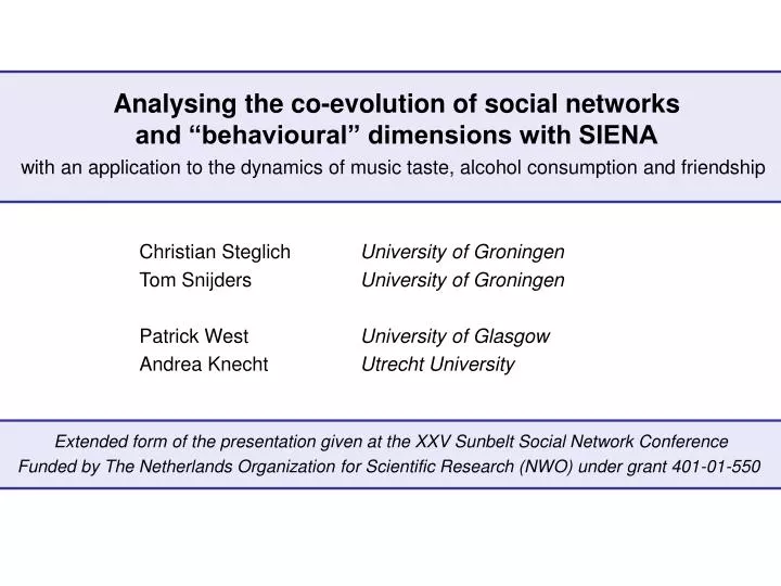
Analysing the co-evolution of social networks and “behavioural” dimensions with SIENA

1. Analysing the co-evolution of social networks • and “behavioural” dimensions with SIENA • Christian Steglich University of Groningen • Tom Snijders University of Groningen • Patrick West University of Glasgow • Andrea Knecht Utrecht University with an application to the dynamics of music taste, alcohol consumption and friendship Extended form of the presentation given at the XXV Sunbelt Social Network Conference Funded by The Netherlands Organization for Scientific Research (NWO) under grant 401-01-550

2. Some notation & clarification • Social networks: • Tie variables • “Behavioural” dimensions: • ...can be any changeable dependent actor variable z i: • overt behaviour • attitudes • cognitions • ... a3 a5 a1 a2 a4

3. Social network dynamics often depend on actors’ characteristics… • – patterns of homophily: • interaction with similar others can be more rewarding than interaction with dissimilar others • – patterns of exchange: • selection of partners such that they complement own abilities • …but also actors’ characteristics can depend on the social network: • – patterns of assimilation: • spread of innovations in a professional community • pupils copying ‘chic’ behaviour of friends at school • traders on a market copying (allegedly) successful behaviour of competitors • – patterns of differentiation: • division of tasks in a work team

4. Example 1: (Andrea Knecht, 2003/04) • Data on the co-evolution of petty delinquency (graffiti, fighting, stealing, • breaking something, buying illegal copies) and friendship among first-grade pupils at Dutch secondary schools (“bridge class”). • 125 school classes • 4 measurement points • Questions to be addressed: • Is petty crime a dimension that plays a role in friendship formation? • Is petty crime a habit that is acquired by peer influence? • The following slides show how the type of data “look like” • that we are analysing. • Note: we analyse panel data – in principle, • continuous-time data is easier to • analyse – but the methods are not • yet implemented.

5. Friendship ties inherited from primary school • girls yellow boys green

6. 1st wave: August/September 2003 node size indicates strength of delinquency

7. 2nd wave: November/December 2003

8. 3rd wave: February/March 2004

9. 4th wave: May/June 2004

10. What do these pictures tell us? • – there is segregation of the friendship network according to gender (although not as strong as in other classes) • – delinquency is stronger among boys than among girls • Questions unanswered: • – to what degree can social influence and social selection processes account for the observed dynamics? • More general…

11. persistence (?) beh(tn) beh(tn+1) selection influence net(tn) net(tn+1) persistence (?) • How to analyse this? • structure of complete networks is complicated to model • additional complication due to the interdependence with behavior • and on top of that often incomplete observation (panel data)

12. Agenda for this talk: • Presentation of the stochastic modelling framework • An illustrative research question (Example 2) • Data for Example 2 • Software • Analysis • Interpretation of results • Summary

13. Brief sketch of the stochastic modelling framework • Stochastic process in the space of all possible network-behaviour configurations • (huge!) • First observation as the process’ starting value. • Change is modelled as occurring in continuous time. • Network actors drive the process: individual decisions. • two domains of decisions*: • decisions about network neighbours (selection, deselection), • decisions about own behaviour. • per decision domain two submodels: • When can actor i make a decision? (rate function) • Which decision does actor i make? (objective function) • Technically: Continuous time Markov process. • Beware: model-based inference! • *assumption: conditional independence, given the current state of the process. beh net

14. How does the model look like? • State space • Pair (x,z)(t) contains adjacency matrix x and vector(s) • of behavioural variables zat time point t. • Stochastic process • Co-evolution is modelled by specifying transition probabilities • between such states (x,z)(t1) and (x,z)(t2). • Continuous time model • invisibility of to-and-fro changes in panel data poses no problem, • evolution can be modelled in smaller units (‘micro steps’). • Observed changes are quite complex – they areinterpreted as resulting from a sequence of micro steps.

15. Micro steps that are modelled explicitly • network micro steps: • (x,z)(t1) and (x,z)(t2) differ in one tie variable xij only. • behavioural micro steps: • (x,z)(t1) and (x,z)(t2) differ (by one) in one behaviouralscore variable zionly. • Actor-driven model • Micro steps are modelled as outcomes of an actor’s decisions; • these decisions are conditionally independent, given the current state of the process. • Schematic overview of model components

16. Timing of decisions / transitions • Waiting times l between decisions are assumed to be exponentially distributed (Markov process); • they can depend on state, actor and time. • Network micro step / network decision by actor i • Choice options • change tie variable to one other actor j • change nothing • Maximize objective function + random disturbance • Choice probabilities resulting from distribution of eare of multinomial logit shape Random part, i.i.d. over x, z, t, i, j, according to extreme value type I Deterministic part, depends on network-behavioural neighbourhood of actor i x(i  j) is the network obtained from x by changing tie to actor j; x(i i) formally stands for keeping the network as is

17. Network micro step / network decision by actor i • Objective function f is linear combination of “effects”, with parameters as effect weights. • Examples: • reciprocity effect • measures the preference difference of actor i between right and left configuration • transitivity effect i j i j j j i i k k

18. Other possible effects to include in the network objective function: • (from Steglich, Snijders & Pearson 2004)

19. Behavioural micro step by actor i • Choice options • increase, decrease, or keep score on behavioural variable • Maximize objective function + random disturbance • Choice probabilities analogous to network part Assume independence also of the network random part Objective function is different from the network objective function

20. Other possible effects to include in the behavioural objective function(s): • (from Steglich, Snijders & Pearson 2004)

21. Modelling selection and influence • Influence and selection are based • on a measure of behavioural similarity • Similarity of actor i to network neighbours : • Actor i hastwo ways of increasing friendship similarity: • by choosing friends j who behave the same (network effect): • by adapting own behaviour to that of friends j (behaviour effect): i j i j homophily (social selection) i j i j i j i j assimilation (social influence) i j i j

22. Total process model • Transition intensities (‘infenitesimal generator’) of Markov process: • Here l = waiting times, d= change in behavioural, • z(i,d) = behavioural vector after change. • Together with starting value, process model is fully defined. • Parametrisation of process implies equilibrium distribution, process is a ‘drift’ from 1st observation towards regions of high probability under this equilibrium.

23. Remarks on model estimation • The likelihood of an observed data set cannot be calculated in closed form, but can at least be simulated. •  ‘third generation problem’ of statistical analysis, •  simulation-based inference is necessary. • Currently available: • Method of Moments estimation (Snijders 2001, 1998) • Maximum likelihood approach (Snijders & Koskinen 2003) • Implementation: program SIENA, part of the StOCNETsoftware package (see link in the end).

24. Example (2): • A set of illustrative research questions: • To what degree is music taste acquired via friendship ties? • Does music taste (co-)determine the selection of friends? • Data: social network subsample of the West of Scotland 11-16 Study • (West & Sweeting 1996) • three waves, 129 pupils (13-15 year old) at one school • pupils named up to 12 friends • Take into account previous results on same data (Steglich, Snijders & Pearson 2004): • What is the role played by alcohol consumption in both friendship formation and the dynamics of music taste?

25. Music question: 16 items 43. Which of the following types of music do you like listening to? Tick one or more boxes. Rock  Indie  Chart music  Jazz  Reggae  Classical  Dance  60’s/70’s  Heavy Metal  House  Techno  Grunge  Folk/Traditional  Rap  Rave  Hip Hop  Other (what?)…………………………………. • Before applying SIENA: data reduction to • the 3 most informative dimensions

26. scale ROCK scale CLASSICAL scale TECHNO

27. Alcohol question: five point scale 32. How often do you drink alcohol? Tick one box only. More than once a week  About once a week About once a month  Once or twice a year I don’t drink (alcohol)  5 4 3 2 1 General: SIENA requires dichotomous networks and behavioural variables on an ordinal scale.

28. Some descriptives: average dynamics of the four behavioural variables global dynamics of friendship ties (dyad counts)

29. Software: The models briefly sketched above are instantiated in the SIENA program. Optionally, evolution models can be estimated from given data, or evolution processes can be simulated, given a model parametrisation and starting values for the process. SIENA is implemented in the StOCNET program package, available at http://stat.gamma.rug.nl/stocnet (release 14-feb-05). Currently, it allows for analysing the co-evolution of one social network (directed or undirected) and multiple behavioural variables.

30. Recoding of variables and identification of missing data Specifying subsets of actors for analyses Identification of data sourcefiles

32. Data specification: insert data into the model’s “slots”.

33. Model specification: select parameters to include for network evolution.

34. Model specification: select parameters to include for behavioural evolution.

35. Model specification: some additional features.

36. Model estimation: stochastic approximation of optimal parameter values.

37. Analysis of the music taste data: • Network objective function: • intercept: • outdegree • network-endogenous: • reciprocity • distance-2 • covariate-determined: • gender homophily • gender ego • gender alter • behaviour-determined: • beh. homophily • beh. ego • beh. alter • Rate functions were kept as simple as possible (periodwise constant). • Behaviour objective function(s): • intercept: • tendency • network-determined: • assimilation to neighbours • covariate-determined: • gender main effect • behaviour-determined: • behaviour main effect • “behaviour” stands shorthand for the three music taste dimensions and alcohol consumption.

38. Results: network evolution Ties to just anyone are but costly. Reciprocated ties are valuable (overcompensating the costs). There is a tendency towards transitive closure. • There is gender homophily: • alter • boy girl • boy0.38 -0.62 • ego • girl-0.18 0.41 • table gives gender-related contributions to the objective function • There is no general homophily according to music taste: • alter • techno rock classical • techno -0.06 0.25 -1.39 • ego rock -0.15 0.54 -1.31 • classical 0.02 0.50 1.73 • table renders contributions to the objective function for highest possible scores & mutually exclusive music tastes • There is alcohol homophily: • alter • low high • low0.36 -0.59 • ego • high-0.59 0.13 • table shows contributions to the objective function for highest / lowest possible scores

39. Results: behavioural evolution • Assimilation to friends occurs: • on the alcohol dimension, • on the techno dimension, • on the rock dimension. • There is evidence for mutual exclusiveness of: • listening to techno and listening to rock, • listening to classical and drinking alcohol. • The classical listeners tend to be girls.

40. Summary: • Does music taste (co-)determine the selection of friends? • Somewhat. • There is no music taste homophily • (possible exception: classical music). • Listening to rock music seems to coincide with popularity, • listening to classical music with unpopularity. • To what degree is music taste acquired via friendship ties? • It depends on the specific music taste: • Listening to techno or rock music is ‘learnt’ from peers, • listening to classical music is not – maybe a ‘parent thing’? • Check out the software at http://stat.gamma.rug.nl/stocnet/