Download

1 / 38
390 likes | 597 Views
fMRI design and analysis. Basic designs. MRI vs. fMRI. Functional MRI (fMRI) studies brain function. MRI studies brain anatomy. MRI vs. fMRI. MRI. fMRI. high resolution (1 mm). low resolution (~3 mm but can be better). one image. …. fMRI

E N D
fMRI design and analysis Basic designs
MRI vs. fMRI Functional MRI (fMRI) studies brain function. MRI studies brain anatomy.
MRI vs. fMRI MRI fMRI high resolution (1 mm) low resolution (~3 mm but can be better) one image … • fMRI • Blood Oxygenation Level Dependent (BOLD) signal • indirect measure of neural activity many images (e.g., every 2 sec for 5 mins) neural activity blood oxygen fMRI signal
fMRI Activation Flickering Checkerboard OFF (60 s) - ON (60 s) -OFF (60 s) - ON (60 s) - OFF (60 s) Brain Activity Time Source: Kwong et al., 1992
fMRI Experiment Stages: Prep • 1) Prepare subject • Consent form • Safety screening • Instructions and practice trials if appropriate • 2) Shimming • putting body in magnetic field makes it non-uniform • adjust 3 orthogonal weak magnets to make magnetic field as homogenous as possible • 3) Sagittals • Take images along the midline to use to plan slices Perhaps the most frequently misspelled word in fMRI: Should have one g, two t’s In this example, these are the functional slices we want: 12 slices x 6 mm
fMRI Experiment Stages: Anatomicals • 4) Take anatomical (T1) images • high-resolution images (e.g., 0.75 x 0.75 x 3.0 mm) • 3D data: 3 spatial dimensions, sampled at one point in time • 64 anatomical slices takes ~4 minutes 64 slices x 3 mm
Slice Terminology VOXEL (Volumetric Pixel) Slice Thickness e.g., 6 mm In-plane resolution e.g., 192 mm / 64 = 3 mm 3 mm 6 mm SAGITTAL SLICE IN-PLANE SLICE 3 mm Number of Slices e.g., 10 Matrix Size e.g., 64 x 64 Field of View (FOV) e.g., 19.2 cm
Coordinates - Anatomy coronal sagittal axial 3 Common Views of Brain: Coronal (head on) Axial (bird’s eye), aka Transverse. Sagittal (profile)
fMRI Experiment Stages: Functionals • 5) Take functional (T2*) images • images are indirectly related to neural activity • usually low resolution images (3 x 3 x 6 mm) • all slices at one time = a volume (sometimes also called an image) • sample many volumes (time points) (e.g., 1 volume every 2 seconds for 136 volumes = 272 sec = 4:32) • 4D data: 3 spatial, 1 temporal …
Activation Statistics ROI Time Course fMRI Signal (% change) ~2s Condition Time Condition 1 Statistical Map superimposed on anatomical MRI image Condition 2 ... Region of interest (ROI) ~ 5 min Functional images Time
Statistical Parametric Map Design matrix fMRI time-series kernel Motion correction Smoothing General Linear Model Spatial normalisation Parameter Estimates Standard template Overview
Spatial Realignment: Reasons for Motion Correction Subjects will always move in the scanner The sensitivity of the analysis depends on the residual noise in the image series, so movement that is unrelated to the subject’s task will add to this noise and hence realignment will increase the sensitivity However, subject movement may also correlate with the task… …in which case realignment may reduce sensitivity (and it may not be possible to discount artefacts that owe to motion) • Realignment (of same-modality images from same subject) involves two stages: • 1. Registration - estimate the 6 parameters that describe the rigid body transformation between each image and a reference image • 2. Reslicing - re-sample each image according to the determined transformation parameters
Motion Correction Algorithms pitch roll yaw Most algorithms assume a rigid body (i.e., that brain doesn’t deform with movement) Align each volume of the brain to a target volume using six parameters: three translations and three rotations Target volume: the functional volume that is closest in time to the anatomical image z translation y translation x translation
Head Motion: Good, Bad,… Slide from Duke course
… and catastrophically bad Slide from Duke course
Nearest Neighbour Linear Full sinc (no alias) Windowed sinc 2. Reslicing Application of registration parameters involves re-sampling the image to create new voxels by interpolation from existing voxels Interpolation can be nearest neighbour (0-order), tri-linear (1st-order), (windowed) fourier/sinc, or nth-order “b-splines”
Temporal Realignment (Slice-Timing Correction) Most functional MRI uses Echo-Planar Imaging (EPI) Each plane (slice) is typically acquired every 3mm normally axial… … requiring ~32 slices to cover cortex (40 to cover cerebellum too) (actually consists of slice-thickness, eg 2mm, and interslice gap, eg 1mm, sometimes expressed in terms of “distance factor”) (slices can be acquired contiguously, eg [1 2 3 4 5 6], or interleaved, eg [1 3 5 2 4 6]) Each plane (slice) takes about ~60ms to acquire… …entailing a typical TR for whole volume of 2-3s Volumes normally acquired continuously (though sometimes gap so that TR>TA) • 2-3s between sampling the BOLD response in the first slice and the last slice (a problem for transient neural activity; less so for sustained neural activity)
Between Modality Co-registration T1 Transm T2 PD PET EPI Useful, for example, to display functional results (EPI) onto high resolution structural image (T1)… …indeed, necessary if spatial normalisation is determined by T1 image Because different modality images have different properties (e.g., relative intensity of gray/white matter), cannot simply minimise difference between images Therefore, use Mutual Information as cost function, rather than squared differences…
DARTEL: Diffeomorphic Registration (SPM8) Grey matter average of 452 subjects Affine Grey matter average of 471 subjects DARTEL
Coordinates - normalization • Different people’s brains look different • ‘Normalizing’ adjusts overall size and orientation Normalized Images Raw Images
Reasons for Smoothing FWHM Gaussian smoothing kernel Potentially increase signal to noise (matched filter theorem) Inter-subject averaging (allowing for residual differences after normalisation) Increase validity of statistics (more likely that errors distributed normally) • Kernel defined in terms of FWHM (full width at half maximum) of filter - usually ~16-20mm (PET) or ~6-8mm (fMRI) of a Gaussian • Ultimate smoothness is function of applied smoothing and intrinsic image smoothness (sometimes expressed as “resels” - RESolvable Elements)
Statistical Parametric Map Design matrix fMRI time-series kernel Motion correction Smoothing General Linear Model Spatial normalisation Parameter Estimates Standard template Overview
General Linear Model… Parametric statistics • one sample t-test • two sample t-test • paired t-test • Anova • AnCova • correlation • linear regression • multiple regression • F-tests • etc… all cases of theGeneral Linear Model
The General Linear Model T-tests, correlations and Fourier analysis work for simple designs and were common in the early days of imaging The General Linear Model (GLM) is now available in many software packages and tends to be the analysis of choice Why is the GLM so great? the GLM is an overarching tool that can do anything that the simpler tests do you can examine any combination of contrasts (e.g., intact - scrambled, scrambled - baseline) with one GLM rather than multiple correlations the GLM allows much greater flexibility for combining data within subjects and between subjects it also makes it much easier to counterbalance orders and discard bad sections of data the GLM allows you to model things that may account for variability in the data even though they aren’t interesting in and of themselves (e.g., head motion) as we will see later in the course, the GLM also allows you to use more complex designs (e.g., factorial designs)
General Linear Model Equation for single (and all) voxels: yj = xj1b1 + … xjLbL + ej ej ~ N(0,s2) yj : data for scan, j = 1…J xjl :explanatory variables / covariates / regressors, l = 1…L bl : parameters / regression slopes / fixed effects ej : residual errors, independent & identically distributed (“iid”) (Gaussian, mean of zero and standard deviation of σ) Equivalent matrix form: y = Xb + e X : “design matrix” / model
Matrix Formulation Equation for scan j Simultaneous equations for scans 1.. J …that can be solved for parameters b1.. L Regressors Scans
A Simple Experiment • Lateral Occipital Complex • responds when subject views objects Blank Screen Intact Objects Scrambled Objects TIME One volume (12 slices) every 2 seconds for 272 seconds (4 minutes, 32 seconds) Condition changes every 16 seconds (8 volumes)
What’s real? A. C. B. D.
What’s real? I created each of those time courses based by taking the predictor function and adding a variable amount of random noise signal = + noise
Linear Drift Huettel, Song & McCarthy, 2004, Functional Magnetic Resonance Imaging
Physiological Noise • Respiration • every 4-10 sec (0.3 Hz) • moving chest distorts susceptibility • Cardiac Cycle • every ~1 sec (0.9 Hz) • pulsing motion, blood changes • Solutions • gating • avoiding paradigms at those frequencies
Low and High Frequency Noise Source: Smith chapter in Functional MRI: An Introduction to Methods
We create a GLM with 2 predictors × 1 = + + × 2 = + fMRI Signal Design Matrix x Betas Residuals “what we CAN explain” “how much of it we CAN explain” “what we CANNOT explain” = x + “our data” Statistical significance is basically a ratio of explained to unexplained variance
Implementation of GLM in SPM Intact Predictor Scrambled Predictor SPM represents time as going down SPM represents predictors within the design matrix as grayscale plots (where black = low, white = high) over time SPM includes a constant to take care of the average activation level throughout each run Many thanks to Øystein Bech Gadmar for creating this figure in SPM Time
Contrasts in the GLM • We can also examine whether a single predictor is significantly greater than another predictor We can examine whether a single predictor is significant (compared to the baseline)