Lecture 3a: Feature detection and matching

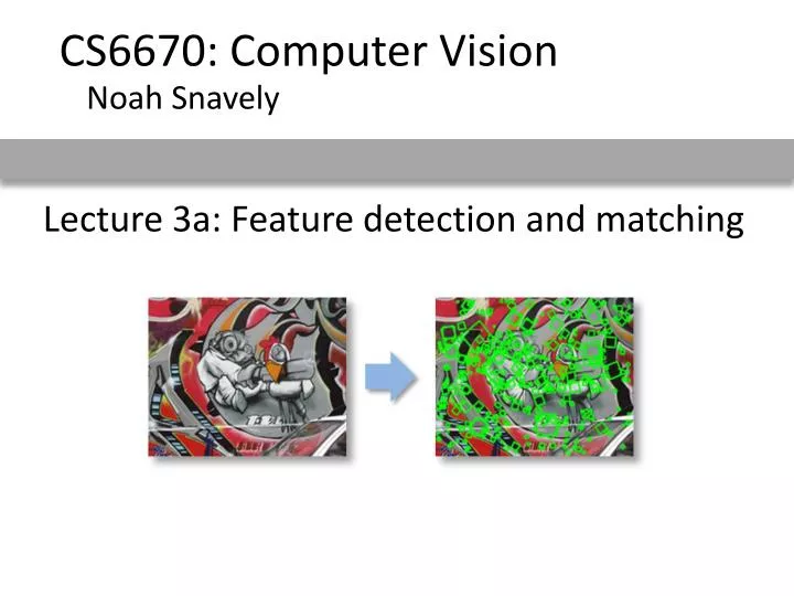
1. CS6670: Computer Vision Noah Snavely Lecture 3a: Feature detection and matching

2. Reading • Szeliski: 4.1

3. Feature extraction: Corners and blobs

4. Motivation: Automatic panoramas Credit: Matt Brown

5. Motivation: Automatic panoramas HD View http://research.microsoft.com/en-us/um/redmond/groups/ivm/HDView/HDGigapixel.htm Also see GigaPan: http://gigapan.org/

6. Why extract features? • Motivation: panorama stitching • We have two images – how do we combine them?

7. Why extract features? • Motivation: panorama stitching • We have two images – how do we combine them? Step 1: extract features Step 2: match features

8. Why extract features? • Motivation: panorama stitching • We have two images – how do we combine them? Step 1: extract features Step 2: match features Step 3: align images

9. Image matching by Diva Sian by swashford TexPoint fonts used in EMF. Read the TexPoint manual before you delete this box.: AAAAAA

10. Harder case by Diva Sian by scgbt

11. Harder still? NASA Mars Rover images

12. Answer below (look for tiny colored squares…) NASA Mars Rover images with SIFT feature matches

13. Feature Matching

14. Feature Matching

15. Invariant local features Find features that are invariant to transformations • geometric invariance: translation, rotation, scale • photometric invariance: brightness, exposure, … Feature Descriptors

16. Advantages of local features Locality • features are local, so robust to occlusion and clutter Quantity • hundreds or thousands in a single image Distinctiveness: • can differentiate a large database of objects Efficiency • real-time performance achievable

17. More motivation… Feature points are used for: • Image alignment (e.g., mosaics) • 3D reconstruction • Motion tracking • Object recognition • Indexing and database retrieval • Robot navigation • … other

18. What makes a good feature? Snoop demo

19. Want uniqueness Look for image regions that are unusual • Lead to unambiguous matches in other images How to define “unusual”?

20. Local measures of uniqueness Suppose we only consider a small window of pixels • What defines whether a feature is a good or bad candidate? Credit: S. Seitz, D. Frolova, D. Simakov

21. Local measure of feature uniqueness • How does the window change when you shift it? • Shifting the window in any direction causes a big change “corner”:significant change in all directions “flat” region:no change in all directions “edge”: no change along the edge direction Credit: S. Seitz, D. Frolova, D. Simakov

22. Harris corner detection: the math • Consider shifting the window W by (u,v) • how do the pixels in W change? • compare each pixel before and after bysumming up the squared differences (SSD) • this defines an SSD “error” E(u,v): W

23. Small motion assumption • Taylor Series expansion of I: • If the motion (u,v) is small, then first order approximation is good • Plugging this into the formula on the previous slide…

24. Corner detection: the math • Consider shifting the window W by (u,v) • define an SSD “error” E(u,v): W

25. Corner detection: the math • Consider shifting the window W by (u,v) • define an SSD “error” E(u,v): W • Thus, E(u,v) is locally approximated as a quadratic error function

26. The second moment matrix The surface E(u,v) is locally approximated by a quadratic form. Let’s try to understand its shape.

27. E(u,v) Horizontal edge: v u

28. E(u,v) Vertical edge: v u

29. direction of the fastest change direction of the slowest change (max)-1/2 (min)-1/2 General case We can visualize H as an ellipse with axis lengths determined by the eigenvalues of H and orientation determined by the eigenvectors of H max,min: eigenvalues of H Ellipse equation:

30. Corner detection: the math xmin xmax • Eigenvalues and eigenvectors of H • Define shift directions with the smallest and largest change in error • xmax = direction of largest increase in E • max = amount of increase in direction xmax • xmin = direction of smallest increase in E • min = amount of increase in direction xmin

31. Corner detection: the math • How are max, xmax, min, and xmin relevant for feature detection? • What’s our feature scoring function?

32. Corner detection: the math • How are max, xmax, min, and xmin relevant for feature detection? • What’s our feature scoring function? • Want E(u,v) to be large for small shifts in all directions • the minimum of E(u,v) should be large, over all unit vectors [u v] • this minimum is given by the smaller eigenvalue (min) of H

33. Interpreting the eigenvalues Classification of image points using eigenvalues of M: 2 “Edge” 2 >> 1 “Corner”1 and 2 are large,1 ~ 2;E increases in all directions 1 and 2 are small;E is almost constant in all directions “Edge” 1 >> 2 “Flat” region 1

34. Corner detection summary • Here’s what you do • Compute the gradient at each point in the image • Create the H matrix from the entries in the gradient • Compute the eigenvalues. • Find points with large response (min> threshold) • Choose those points where min is a local maximum as features

35. Corner detection summary • Here’s what you do • Compute the gradient at each point in the image • Create the H matrix from the entries in the gradient • Compute the eigenvalues. • Find points with large response (min> threshold) • Choose those points where min is a local maximum as features

36. The Harris operator • min is a variant of the “Harris operator” for feature detection • The trace is the sum of the diagonals, i.e., trace(H) = h11 + h22 • Very similar to min but less expensive (no square root) • Called the “Harris Corner Detector” or “Harris Operator” • Lots of other detectors, this is one of the most popular

37. The Harris operator Harris operator

38. Harris detector example

39. f value (red high, blue low)

40. Threshold (f > value)

41. Find local maxima of f

42. Harris features (in red)

43. Weighting the derivatives • In practice, using a simple window W doesn’t work too well • Instead, we’ll weight each derivative value based on its distance from the center pixel

44. Questions?