Download
1 / 23
270 likes | 442 Views
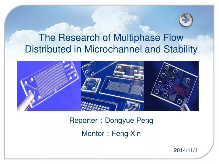
The Research of Multiphase Flow Distributed in Microchannel and Stability. Reporter : Dongyue Peng Mentor : Feng Xin. Contents. Introduction. Goals. Relevant references. Flow resistance model and nonlinear dynamic system. Next plan. Introduction. 1. What is microchannel ?

E N D
The Research of Multiphase Flow Distributed in Microchannel and Stability Reporter:Dongyue Peng Mentor:Feng Xin
Contents Introduction Goals Relevant references Flow resistance model and nonlinear dynamic system Next plan
Introduction 1 What is microchannel ? Microchannel isfabricated by micromachining and precision machining technology. The dimension of channel cross-section is 0.5mm(500um) or less, which makes it different from others. Advantage: 1、Have a largespecific surface 2、Enhancing heat and mass transfer progress 3、less reagents 4、Much saferand easier to control 5、Numbering-up
Introduction 1 Compared to the traditional approach of scale up, numbering-up avoids the route from laboratory-scale to pilot plant scale to commercial plant. However, one key challenge of numbering up is non-uniformity flow distributed in microchannel . Reason:there exists feedback among these channels and this feedback combined with the amplification of a slight difference in resistances of these channels. This negative effect leads to non-uniformity ,sometimes, even chaotic disturbance . Fig. 1. Photos of CO2 -water flow pattern in 16 parallel microchannels Adopted from Yue. Boichot et al. (2009)
Goals 2 1、Present a valid model ormethod to describe the microchannel system, which can explain the ratio of fluid in each channel and flow state(stable, periodic, or chaos). 2、Introduce some disturbances into the system and study its capacity to resist the interference. Fig. 2. Schematic view of ideal description flow distribution Fig. 3. schematic view when introducing external interference
Relevant references 3 B A Fig. 4. Schematic representation of gas–liquid flow distribution over parallel microchannels:(A)external distribution (B) internal distribution . Adopted from Al-Rawashdeh ,M et al.(2012).
Analysis of the microchannel 2 A B Fig. 5. Photos of CO2-water flow pattern in 16 parallel microchannels (A) low speed of gaseous phase (B) high speed of gaseous phase. Adopted from Yue ,Boichot et al.(2009) the Multi-phase flow in microchannel results in different flow regimes. Among them, taylor flow is attractive due to its well defined gas-liquid interface reduced axial dispersion approaching ideal plug flow, and its excellent mass transfer and heat transfer characteristics.
Relevant references 3 B A C Fig. 6. (A) Schematic representation of barrier-based gas–liquid flow distributor for four parallel microchannels. Adopted from Al-Rawashdeh, Fluitsma et al.(2012) (B) Schematic of the distribution unit with a PTFE. Adoped from Matthias Mendorf et al.(2010) (C) Schematic view of the railroad-like channel network. Adopted from Ahn, Lee et al.(2011)
Relevant references 3 A B Fig. 7. The selection of paths by bubbles, at multiple bubble density levels. Adopted from Choi,Hashimoto et al. (2011) A micrograph of the experimental setup and a graph of the mean ratio of the numbers of drop-lets traveling through each of the two arms of the loops. Adopted from Jousse, Farr et al.(2006)
Resistance model 4 A B Fig. 8. Simplified resistance network model. Adopted from Pan, M., Y. Tang, et al. (2009). Schematic view for gas–liquid flow in multiple parallel microchannels. Adopted from Al-Rawashdeh, Fluitsma et al.(2012) Fundamental formula ΔP = R×Q
Resistance model 4 Fig. 9. Schematic view for gas–liquid flow in multi-parallel microchannels. Fundamental Assumptions: 1 fixed physical properties; 2 the pressure of outlet equals to atmosphere; 3 ignore pressure drop when two phases mix 4 Only consider the influence of channel size on the fluid distribution
Resistance model 4 Rl1 Ql1+ Rm1(Ql1+ Qg1)= Rl2 Ql2+ Rm2(Ql2+ Qg2) Rg1 Qg1+ Rm1(Ql1+ Qg1)= Rg2 Qg2+ Rm2(Ql2+ Qg2) Ql1+ Ql2=Ql Qg1+ Qg2=Qg P-P0=P-P0 (Ql1, Ql2, Qg1, Qg2,) Table.1.Experimental parameter ( 25℃)
Resistance model 4 start Input physical properties and flow rates Input the size of channels Assumed Rm1=0,Rm2=0,calculated Rl1,Rl2,Rg1,Rg2,then calculate initial value Ql1, Ql2, Qg1,Qg2. Choose the valid model to calculate Rm1,Rm2 According to the pressure equilibrium, calculate value Ql1, Ql2, Qg1,Qg2 again. Yes Calculate multiphase flow distribution end Fig. 9. Sequence procedures for solving the resistance model.
Resistance model 4 To ensure an accurate result, the key of the progress is to choose a valid and accurate model to calculate Rm1 and Rm2 HFM model and SFM model SFM : Adopted from Choi and Kim et al. (2011) Bubble model Adopted from Fuerstman, Lai et al.(2007)
Resistance model 4 Table.2. Experimental Variables
Resistance model 4 A B C Conclusion: 1 Gas-phase of fluid distributed in channel is much more sensitive to the changed size of liquid channel than that of gas channel. 2 The deviation from height contributes more to non-uniform distribution than that from the width. 3 On the same deviation, the distribution of liquid is more uniform than that of gas 4 The influence of manufacturing tolerance should be care more. Fig. 10. the relationship of channel size and gas phase flow distributuion:(A)change the width of liquid and gas channel,(B) change the width of gas channel and height of liquid channel,(C) change the height of liquid and gas channel.
Resistance model 4 A B C Conclusion 1 The result of bubble model is a little bigger than that of SFM model. 2 Decrease the rate of gas, the deviation will enlarge. Fig. 11. the relationship of channel size and gas phase flow distribution:(A)change the width of liquid and gas channel in SFM model (B) change the width of gas and liquid channel in Bubble model, (C) change the width of liquid and gas channel in a smaller flow rate of gas.
Resistance model 4 The progress of iteration is always non-convergence Initial value of Ql1, Ql2 Qg1 Qg2 Output the value of Ql1, Ql2 Qg1 Qg2 Fig. 12. Schematic view of iteration procedure. Fig. 13. The value of flow rate during iteration
Nonlinear dynamic system 4 In our nature, almost everything have relationship with each other and most of these relationships are nonlinear, like the butterfly effect. In my opinion, the application of nonlinear dynamical systemcan be divided into two classes, one of which adopts chaotic time series. We can obtain the Largest Lyapunov exponent, fractiondimension,Kolmogorov entropy and phase diagram and so on, which can ensure us a systematic system analysis and prediction. (Schembri,Sapuppo et al.2011) Another method is applying existed equations to represent the nonlinear system. That is to say, It mainly relies on the experimental data to obtain related equation parameters. (Barbier, Willaime et al.2006)
Nonlinear dynamic system 4 The discrete conditions of chaos are often performed by chaotic time series, and this chaotic time series contains a plenty of system dynamic information. A D B C Fig. 13. (A) Time series for Vair=0.12ml/min,V water=0.63ml/min and for Vair=1.2ml/min,Vwater=6.3ml/min (B) Schematic of a microfluidic snake channel.(C) contour plot of Largest Lyapunov exponent versus Air Fraction (D) Phase diagrams for Vair = 7.43 ml/min, Vwater = 1.57 ml/min and for Vair = 0.17 ml/min, Vwater = 0.15 ml/min. Adopt from Schembri, Sapuppo et al.(2001)
Nonlinear dynamic system 4 A B Fig. 13. (A) Sketch of the parallelized system,(B) Dynamic behaviors in two microfluids with different flow rate: (a) Qo=4 L/min,Qw=0.6 L/min, Qw’ =0.5 L/min; (b) Qo=4 L/min, Qw=1.2 L/min, Qw ’ =0.5 L/min. Adopted from Barbier, Willaime et al. (2006)
Next plan 5 1 、A lot of improvements should consider in order to design a more accurate model . It should consider pressure value of the bubbles and two phases mix. After that , the influence coming from feedback should be added in the model. 2、Attempt to use the method of nonlinear dynamic system to describe the microchannel system, and then make some accurate predictions. 3、 Wish to verify some assumptions by experiment, like the actual situation of flow disturbance and the its capacity to resist the interference.