Download
1 / 107
1.12k likes | 1.42k Views
Numerical Descriptive Techniques. Chapter 4. Introduction. Recall Chapter 2, where we used graphical techniques to describe data:. While this histogram provides some new insight, other interesting questions (e.g. what is the class average? what is the mark spread?) go unanswered.

E N D
Numerical Descriptive Techniques Chapter 4
Introduction • Recall Chapter 2, where we used graphical techniques to describe data: • While this histogram provides some new insight, other interesting questions (e.g. what is the class average? what is the mark spread?) go unanswered.
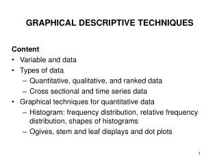
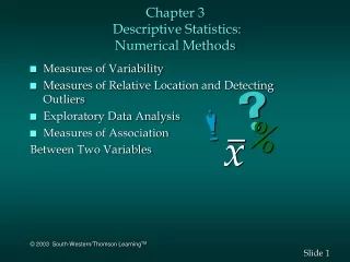
Numerical Descriptive Techniques • Measures of Central Location(中央位置) • Mean, Median, Mode • Measures of Variability(離散程度) • Range, Standard Deviation, Variance, Coefficient of Variation • Measures of Relative Standing(相對位置) • Percentiles, Quartiles • Measures of Linear Relationship(線性關係) • Covariance, Correlation, Least Squares Line
4.1 Measures of Central Location • Usually, we focus our attention on two types of measures when describing population characteristics: • Central location (e.g. average) • Variability or spread The measure of central location reflects the locations of all the actual data points.
With one data point clearly the central location is at the point itself. 4.1 Measures of Central Location • The measure of central location reflects the locations of all the actual data points. • How? With two data points, the central location should fall in the middle between them (in order to reflect the location of both of them). But if the third data point appears on the left hand-side of the midrange, it should “pull” the central location to the left.
Sum of the observations Number of observations Mean = The Arithmetic Mean(算術平均數) • This is the most popular and useful measure of central location
Notation • When referring to the number of observations in a population, we use uppercase letter N • When referring to the number of observations in a sample, we use lower case letter n • The arithmetic mean for a population is denoted with Greek letter “mu”: (母體平均數) • The arithmetic mean for a sample is denoted with an “x-bar”.(樣本平均數)
The Arithmetic Mean Sample mean Population mean Sample size Population size
Example 4.2 Suppose the telephone bills of Example 2.1 represent the populationof measurements. The population mean is The Arithmetic Mean • Example 4.1 The reported time on the Internet of 10 adults are 0, 7, 12, 5, 33, 14, 8, 0, 9, 22 hours. Find the mean time on the Internet. 0 7 22 11.0 42.19 38.45 45.77 43.59
When many of the measurements have the same value, the measurement can be summarized in a frequency table. Suppose the number of children in a sample of 16 employees were recorded as follows: Number of children per family 0 1 2 3 Number of families 3 4 7 2 + + + 16 employees The Arithmetic Mean • Additional Example
The Arithmetic Mean • …is appropriate for describing measurement data, e.g. heights of people, marks of student papers, etc. • …is seriously affected by extreme values called “outliers”. E.g. as soon as a billionaire moves into a neighborhood, the average household income increases beyond what it was previously!
Example 4.3 Find the median of the time on the internetfor the 10 adults of example 4.1 Suppose only 9 adults were sampled (exclude, say, the longest time (33)) Comment Even number of observations 0, 0, 5, 7, 8,9, 12, 14, 22, 33 The Median(中位數) • The Median of a set of observations is the value that falls in the middle when the observations are arranged in order of magnitude. Odd number of observations 8 8.5, 0, 0, 5, 7, 89, 12, 14, 22 0, 0, 5, 7, 8,9, 12, 14, 22, 33
The modal class The Mode(眾數) • The Mode of a set of observations is the value that occurs most frequently. • Set of data may have one mode (or modal class), or two or more modes. For large data sets the modal class is much more relevant than a single-value mode.
The Mode • Example 4.5Find the mode for the data in Example 4.1. Here are the data again: 0, 7, 12, 5, 33, 14, 8, 0, 9, 22 Solution • All observation except “0” occur once. There are two “0”. Thus, the mode is zero. • Is this a good measure of central location? • The value “0” does not reside at the center of this set(compare with the mean = 11.0 and the mode = 8.5).
The Mode • Additional example • The manager of a men’s store observes the waist size (in inches) of trousers sold yesterday: 31, 34, 36, 33, 28, 34, 30, 34, 32, 40. • The mode of this data set is 34 in. This information seems to be valuable (for example, for the design of a new display in the store), much more than “ the median is 33.5 in.”
Measures of Central Location • The mode of a set of observations is the value that occurs most frequently. • A set of data may have one mode (or modal class), or two, or more modes. • Mode is a useful for all data types, though mainly used for nominal data. • For large data sets the modal class is much more relevant than a single-value mode. ※ Sample and population modes are computed the same way.
=MODE(range) in Excel • Note: if you are using Excel for your data analysis and your data is multi-modal (i.e. there is more than one mode), Excel only calculates the smallest one. • You will have to use other techniques (i.e. histogram) to determine if your data is bimodal, trimodal, etc.
The Mean, Median and Mode • Additional example A professor of statistics wants to report the results of a midterm exam, taken by 100 students. • The mean of the test marks is 73.90 • The median of the test marks is 81 • The mode of the test marks is 84 Describe the information each one provides. The mean provides information about the over-all performance level of the class. It can serve as a tool for making comparisons with other classes and/or other exams. The Median indicates that half of the class received a grade below 81%, and half of the class received a grade above 81%. A student can use this statistic to place his mark relative to other students in the class. The mode must be used when data are nominal If marks are classified by letter grade, the frequency of each grade can be calculated. Then, the mode becomes a logical measure to compute.
Relationship among Mean, Median, and Mode • If a distribution is symmetrical, the mean, median and mode coincide • If a distribution is asymmetrical, and skewed to the left or to the right, the three measures differ. A positively skewed distribution (“skewed to the right”) Mode Mean Median
Relationship among Mean, Median, and Mode • If a distribution is symmetrical, the mean, median and mode coincide • If a distribution is non symmetrical, and skewed to the left or to the right, the three measures differ. A negatively skewed distribution (“skewed to the left”) A positively skewed distribution (“skewed to the right”) Mode Mean Mean Mode Median Median
Mean, Median, Mode • If data are symmetric, the mean, median, and mode will be approximately the same. • If data are multimodal, report the mean, median and/or mode for each subgroup. • If data are skewed, report the median.
Mean, Median, & Modes for Ordinal & Nominal Data • For ordinal and nominal data the calculation of the mean is not valid. • Median is appropriate for ordinal data. • For nominal data, a mode calculation is useful for determining highest frequency but not“central location”.
The Geometric Mean(幾何平均數) • This is a measure of the average growth rate. • Let Ri denote the the rate of return in period i (i=1,2…,n). The geometric mean of the returns R1, R2, …,Rn is the constant Rgthat produces the same terminal wealth at the end of period n as do the actual returns for the n periods.
The Geometric Mean For the given series of rate of returns the nth period return is calculated by: If the rate of return was Rg in every period, the nth period return would be calculated by: = Rg is selected such that…
Finance Example • Suppose a 2-year investment of $1,000 grows by 100% to $2,000 in the first year, but loses 50% from $2,000 back to the original $1,000 in the second year. What is your average return? • Using the arithmetic mean, we have • This would indicate we should have $1,250 at the end of our investment, not $1,000. • Solving for the geometric mean yields a rate of 0%, which is correct. The upper case Greek Letter “Pi” represents a product of terms…
The Geometric Mean • Additional Example • A firm’s sales were $1,000,000 three years ago. • Sales have grown annually by 20%, 10%, -5%. • Find the geometric mean rate of growth in sales. • Solution • Since Rg is the geometric mean (1+Rg)3 = (1+.2)(1+.1)(1-.05)= 1.2540 Thus,
Measures of Central Location: Summary • Compute the Mean to • Describe the central location of a single set of interval data • Compute the Median to • Describe the central location of a single set of interval or ordinal data • Compute the Mode to • Describe a single set of nominal data • Compute the Geometric Mean to • Describe a single set of interval data based on growth rates
4.2 Measures of variability • Measures of central location fail to tell the whole story about the distribution. • A question of interest still remains unanswered: How much are the observations spread out around the mean value?
4.2 Measures of variability Observe two hypothetical data sets: Small variability The average value provides a good representation of the observations in the data set. This data set is now changing to...
4.2 Measures of variability Observe two hypothetical data sets: Small variability The average value provides a good representation of the observations in the data set. Larger variability The same average value does not provide as good representation of the observations in the data set as before.
Measures of Variability • Measures of central location fail to tell the whole story about the distribution; that is, how much are the observations spread out around the mean value? For example, two sets of class grades are shown. The mean (=50) is the same in each case… But, the red class has greater variability than the blue class.
? ? ? The range(全距) • The range of a set of observations is the difference between the largest and smallest observations. • Its major advantage is the ease with which it can be computed. • Its major shortcoming is its failure to provide information on the dispersion of the observations between the two end points. But, how do all the observations spread out? The range cannot assist in answering this question Range Largest observation Smallest observation
Range • The range is the simplest measure of variability, calculated as: • Range = Largest observation – Smallest observation • E.g. • Data: {4, 4, 4, 4, 50} Range = 46 • Data: {4, 8, 15, 24, 39, 50} Range = 46 • The range is the same in both cases, • but the data sets have very different distributions…
Range • Its major advantage is the ease with which it can be computed. • Its major shortcoming is its failure to provide information on the dispersion of the observations between the two end points. • Hence we need a measure of variability that incorporates all the data and not just two observations. Hence…
Variance(變異數) • Variance and its related measure, standard deviation, are arguably the most important statistics. Used to measure variability, they also play a vital role in almost all statistical inference procedures. • Population variance is denoted by (母體變異數) • (Lower case Greek letter “sigma” squared) • Sample variance is denoted by (樣本變異數) • (Lower case “S” squared)
This measure reflects the dispersion of all the observations • The variance of a population of size N x1, x2,…,xN whose mean is m is defined as • The variance of a sample of n observationsx1, x2, …,xn whose mean is is defined as The Variance
The Variance • Example 4.7 • The following sample consists of the number of jobs six students applied for: 17, 15, 23, 7, 9, 13. Finds its mean and variance • Solution
Sum = 0 Sum = 0 Why not use the sum of deviations? Consider two small populations: 9-10= -1 A measure of dispersion Should agrees with this observation. 11-10= +1 Can the sum of deviations Be a good measure of dispersion? The sum of deviations is zero for both populations, therefore, is not a good measure of dispersion. 8-10= -2 A 12-10= +2 8 9 10 11 12 …but measurements in B are more dispersed then those in A. The mean of both populations is 10... 4-10 = - 6 16-10 = +6 B 7-10 = -3 13-10 = +3 4 7 10 13 16
The Variance Let us calculate the variance of the two populations Why is the variance defined as the average squared deviation? Why not use the sum of squared deviations as a measure of variation instead? After all, the sum of squared deviations increases in magnitude when the variation of a data set increases!!
The Variance Which data set has a larger dispersion? Data set B is more dispersed around the mean A B 1 2 3 1 3 5 Let us calculate the sum of squared deviations for both data sets.
SumA = (1-2)2 +…+(1-2)2 +(3-2)2 +… +(3-2)2= 10 SumB = (1-3)2 + (5-3)2 = 8 The Variance SumA > SumB. This is inconsistent with the observation that set B is more dispersed. A B 1 3 1 2 3 5
The Variance However, when calculated on “per observation” basis (variance), the data set dispersions are properly ranked. sA2 = SumA/N = 10/10 = 1 sB2 = SumB/N = 8/2 = 4 A B 1 3 1 2 3 5
Standard Deviation(標準差) • The standard deviation of a set of observations is the square root of the variance .
Standard Deviation • Example 4.8 • To examine the consistency of shots for a new innovative golf club, a golfer was asked to hit 150 shots, 75 with a currently used (7-iron) club, and 75 with the new club. • The distances were recorded. • Which 7-iron is more consistent?
Standard Deviation • Example 4.8 – solution Excel printout, from the “Descriptive Statistics” sub-menu. The innovation club is more consistent, and because the means are close, is considered a better club