Download
1 / 10
100 likes | 326 Views
Chap. 11. PARTIAL DIFFERENTIAL EQUATIONS. An equation involving partial derivatives of an unknown function of two more independent variables PDE Classification of PDES Linear and nonlinear PDEs

E N D
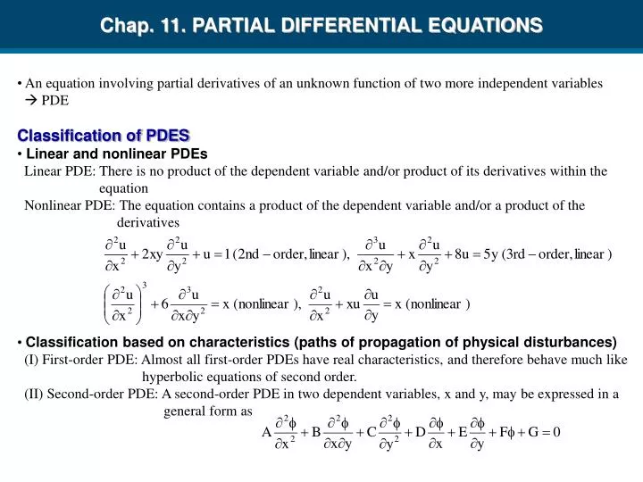
Chap. 11. PARTIAL DIFFERENTIAL EQUATIONS • An equation involving partial derivatives of an unknown function of two more independent variables • PDE • Classification of PDES • Linear and nonlinear PDEs • Linear PDE: There is no product of the dependent variable and/or product of its derivatives within the • equation • Nonlinear PDE: The equation contains a product of the dependent variable and/or a product of the • derivatives • Classification based on characteristics (paths of propagation of physical disturbances) • (I) First-order PDE: Almost all first-order PDEs have real characteristics, and therefore behave much like • hyperbolic equations of second order. • (II) Second-order PDE: A second-order PDE in two dependent variables, x and y, may be expressed in a • general form as
The equation is classified according to the expression (B2-4AC) as follows: • (B2-4AC) < 0 Elliptic equation • = 0 Parabolic equation • > 0 Hyperbolic equation • (a) Elliptic equations • No real characteristic lines exist • A disturbance propagates in all directions • Domain of solution is a closed region • Boundary conditions must be specified on the boundaries of the domain • (b) Parabolic equations • Only one characteristic line exists • A disturbance propagates along the characteristic line • Domain of solution is an open region • An initial condition and two boundary conditions are required • (c) Hyperbolic equations • Two characteristic lines exist • A disturbance propagates along the characteristic lines • Domain of solution is an open region • Two initial conditions along with two boundary conditions are required • Boundary conditions • (a) Dirichlet B.C. (=Essential B.C.): The value of the dependent variable along the boundary is specified • (b) Neumann B.C (=Natural B.C.): The normal gradient of the dependent variable along with the • boundary is specified • (c) Mixed B.C. (Robbin B.C.): A combination of the Dirichlet and the Neumann type B.C.’s is specified
11.1. Basic Concepts • - Linear & nonlinear • - Homogeneous & nonhomogeneous • Ex.1) Important linear 2nd-order PDEs • Theorem 1: Superposition or linearity principle • u1, u2: solutions of a linear homogeneous PDE in R, then • u = c1u1 + c1 u2 : also solution of that equation in R • Ex. 1) A solution u(x,y) of PDE uxx-u=0 • u(x,y) = A(y)ex + B(y)e-x • Ex. 2) PDE uxy = -ux • ux = p py=-p: p=c(x)e-y u(x,y) = f(x)e-y + g(y) where 1D wave Eqn. 1D heat Eqn. 2D Poisson Eqn. 2D Laplace Eqn. 3D Laplace Eqn. 2D wave Eqn.
11.2. Modeling: Vibrating String, Wave Equation - Equation governing small transverse vibration of an elastic string Find the deflection u(x,t): Assumptions: - Constant mass/unit length, perfect elastic, no resistance to bending - Negligible gravitational force - Small transverse motion in vertical plane vertical movement Derivation of the PDE from forces In horizontal direction: In vertical direction: 1D Wave Equation: 2nd-order Hyperbolic PDE
11.3. Separation of Variables: Use of Fourier Series - 1D Wave equation: 2 B.C.’s: u(0,t) = u(L,t) = 0 for all t 2 I.C.’s : u(x,0) = f(x), Solving Steps:- Method of separation variables leading to two ODEs. - Solutions of two eqns. satisfying B.C’s - Final solution of wave eqn. satisfying I.C’s, using Fourier series First Step: Two ODEs using method of separation variables - u(x,t) = F(x)G(t) Second Step: Satisfying the B.C.’s - u(0,t) = F(0)G(t) = 0 Case 1) G = 0 u = 0 (G0) Case 2) k=0 F=0 (k0) u(L,t) = F(L)G(t) = 0 Case 3) k=2 F=0 k = -p2 (negative) Initial velocity Initial deflection (derivative w.r.t t) (derivative w.r.t x) (linear system)
Solving F(x): Solving G(t): Un: harmonic motion with frequency n/2=cn/2L (nth normal mode) nth normal mode has n-1 nodes Tuning controlled by tension T (or c2=T/) (p=n/L) (n: eigenvalues or characteristic values) (Eigenfunctions or characteristic functions) Standing wave solutions
Third Step: Solution to the Entire Problem. Fourier Series • - Sum of many solutions un satisfying I.C.’s: • Satisfying I.C.1: initial displacement (u(x,0) = f(x)) • - Satisfying I.C.2:initial velocity • - Solution (I): for the simple case of g(x) = 0 (Fourier sine series) (Fourier sine series) (f*: odd periodic extension of f with period 2L)
Odd periodic extension of f(x) Physical Interpretation of the Solution f*(x - ct): a wave traveling to the right as t increases constant along each line x - ct f*(x + ct): a wave traveling to the left as t increases constant along each line x + ct c: wave velocity u(x,t): superposition of above two waves Ex. 1) Vibrating string if the initial deflection is triangular. See Ex. 3 in Sec. 10.4 t characteristic lines L/3 x 0 L
Solution (II): for the case of f(x)=0 Solution (III): for the general case of f(x)0 and g(x)0 Exercise: Find the solution of the wave equation with following B.C.’s & I.C.’s utt = c2uxx B.C.’s: ux(0,t) = ux(,t) = 0 for all t I.C.’s: u(x,0) = f(x), ut(x,0) = g(x) (use Fourier cosine series)
11.4. D’Alembert’s Solution of the Wave Equation - Other method to obtain the solution of the wave eqn. u(x,t) u(v,z) usingv = x + ct, z = x – ct D’Alembert Solution Satisfying the Initial Conditions (D’Alembert’s solution) if g(s)=0