Download
1 / 88
880 likes | 1.04k Views
CPS216: Advanced Database Systems Notes 06:Query Execution (Sort and Join operators). Shivnath Babu. SQL query. parse. parse tree. Query rewriting. statistics. logical query plan. Physical plan generation. physical query plan. execute. result. Query Processing - In class order.

E N D
CPS216: Advanced Database SystemsNotes 06:Query Execution (Sort and Join operators) Shivnath Babu
SQL query parse parse tree Query rewriting statistics logical query plan Physical plan generation physical query plan execute result Query Processing - In class order 2; 16.1 3; 16.2,16.3 4; 16.4—16.7 1; 13, 15
Roadmap • A simple operator: Nested Loop Join • Preliminaries • Cost model • Clustering • Operator classes • Operator implementation (with examples from joins) • Scan-based • Sort-based • Using existing indexes • Hash-based • Buffer Management • Parallel Processing
Nested Loop Join (NLJ) R1 R2 • NLJ (conceptually) for each r R1 do for each s R2 do if r.C = s.C then output r,s pair
Nested Loop Join (contd.) • Tuple-based • Block-based • Asymmetric
Implementing Operators • Basic algorithm • Scan-based (e.g., NLJ) • Sort-based • Using existing indexes • Hash-based (building an index on the fly) • Memory management- Tradeoff between memory and #IOs - Parallel processing
Roadmap • A simple operator: Nested Loop Join • Preliminaries • Cost model • Clustering • Operator classes • Operator implementation (with examples from joins) • Scan-based • Sort-based • Using existing indexes • Hash-based • Buffer Management • Parallel Processing
Operator Cost Model • Simplest: Count # of disk blocks read and written during operator execution • Extends to query plans • Cost of query plan = Sum of operator costs • Caution: Ignoring CPU costs
Assumptions • Single-processor-single-disk machine • Will consider parallelism later • Ignore cost of writing out result • Output size is independent of operator implementation • Ignore # accesses to index blocks
Parameters used in Cost Model B(R) = # blocks storing R tuples T(R) = # tuples in R V(R,A) = # distinct values of attr A in R M = # memory blocks available
Roadmap • A simple operator: Nested Loop Join • Preliminaries • Cost model • Clustering • Operator classes • Operator implementation (with examples from joins) • Scan-based • Sort-based • Using existing indexes • Hash-based • Buffer Management • Parallel Processing
Notions of clustering • Clustered file organization ….. • Clustered relation ….. • Clustering index R1 R2 S1 S2 R3 R4 S3 S4 R1 R2 R3 R4 R5 R5 R7 R8
Clustering Index Tuples with a given value of the search key packed in as few blocks as possible 10 10 35 A index 19 19 19 19 42 37
Examples T(R) = 10,000 B(R) = 200 If R is clustered, then # R tuples per block = 10,000/200 = 50 Let V(R,A) = 40 • If I is a clustering index on R.A, then # IOs to access σR.A = “a”(R) = 250/50 = 5 • If I is a non-clustering index on R.A, then # IOs to access σR.A = “a”(R) = 250 ( > B(R))
Roadmap • A simple operator: Nested Loop Join • Preliminaries • Cost model • Clustering • Operator classes • Operator implementation (with examples from joins) • Scan-based • Sort-based • Using existing indexes • Hash-based • Buffer Management • Parallel Processing
Implementing Tuple-at-a-time Operators • One pass algorithm: • Scan • Process tuples one by one • Write output • Cost = B(R) • Remember: Cost = # IOs, and we ignore the cost to write output
Implementing a Full-Relation Operator, Ex: Sort • Suppose T(R) x tupleSize(R) <= M x |B(R)| • Read R completely into memory • Sort • Write output • Cost = B(R)
Implementing a Full-Relation Operator, Ex: Sort • Suppose R won’t fit within M blocks • Consider a two-pass algorithm for Sort; generalizes to a multi-pass algorithm • Read R into memory in M-sized chunks • Sort each chunk in memory and write out to disk as a sorted sublist • Merge all sorted sublists • Write output
1 2 3 4 5 Two-phase Sort: Phase 1 Suppose B(R) = 1000, R is clustered, and M = 100 1 96 1 100 2 97 101 200 3 98 4 99 201 300 5 100 Memory Sorted Sublists 999 801 900 1000 901 1000 R
1 2 3 4 5 Two-phase Sort: Phase 2 100 1 1 200 101 2 3 300 201 4 5 Sorted Sublists 6 7 8 999 900 801 9 1000 10 1000 901 Memory Sorted R
Analysis of Two-Phase Sort • Cost = 3xB(R) if R is clustered, = B(R) + 2B(R’) otherwise • Memory requirement M >= B(R)1/2
Duplicate Elimination • Suppose B(R) <= M and R is clustered • Use an in-memory index structure • Cost = B(R) • Can we do with less memory? • B((R)) <= M • Aggregation is similar to duplicate elimination
Duplicate Elimination Based on Sorting • Sort, then eliminate duplicates • Cost = Cost of sorting + B(R) • Can we reduce cost? • Eliminate duplicates during the merge phase
Back to Nested Loop Join (NLJ) R S • NLJ (conceptually) for each r R do for each s S do if r.C = s.C then output r,s pair
Analysis of Tuple-based NLJ • Cost with R as outer = T(R) + T(R) x T(S) • Cost with S as outer = T(S) + T(R) x T(S) • M >= 2
Block-based NLJ • Suppose R is outer • Loop: Get the next M-1 R blocks into memory • Join these with each block of S • B(R) + (B(R)/M-1) x B(S) • What if S is outer? • B(S) + (B(S)/M-1) x B(R)
Tuple-based NLJ Cost: for each R1 tuple: [Read tuple + Read R2] Total =10,000 [1+5000]=50,010,000 IOs Let us work out an NLJ Example • Relations are not clustered • T(R1) = 10,000 T(R2) = 5,000 10 tuples/block for R1; and for R2 M = 101 blocks
Can we do better when R,S are not clustered? Use our memory (1) Read 100 blocks worth of R1 tuples (2) Read all of R2 (1 block at a time) + join (3) Repeat until done
Cost: for each R1 chunk: Read chunk: 1000 IOs Read R2: 5000 IOs Total/chunk = 6000 Total = 10,000 x 6000 = 60,000 IOs 1,000 [Vs. 50,010,000!]
Reverse join order: R2 R1 Total = 5000 x (1000 + 10,000) = 1000 5 x 11,000 = 55,000 IOs Can we do better? [Vs. 60,000]
Cost For each R2 chunk: Read chunk: 100 IOs Read R1: 1000 IOs Total/chunk = 1,100 Total= 5 chunks x 1,100 = 5,500 IOs Example contd. NLJ R2 R1 • Now suppose relations are clustered [Vs. 55,000]
Joins with Sorting • Sort-Merge Join (conceptually) (1) if R1 and R2 not sorted, sort them (2) i 1; j 1; While (i T(R1)) (j T(R2)) do if R1{ i }.C = R2{ j }.C then OutputTuples else if R1{ i }.C > R2{ j }.C then j j+1 else if R1{ i }.C < R2{ j }.C then i i+1
Procedure Output-Tuples While (R1{ i }.C = R2{ j }.C) (i T(R1)) do [jj j; while (R1{ i }.C = R2{ jj }.C) (jj T(R2)) do [output pair R1{ i }, R2{ jj }; jj jj+1 ] i i+1 ]
Example i R1{i}.C R2{j}.C j 1 10 5 1 2 20 20 2 3 20 20 3 4 30 30 4 5 40 30 5 50 6 52 7
Block-based Sort-Merge Join • Block-based sort • Block-based merge
1 2 3 4 5 Two-phase Sort: Phase 1 Suppose B(R) = 1000 and M = 100 1 96 1 100 2 97 101 200 3 98 4 99 201 300 5 100 Memory Sorted Sublists 999 801 900 1000 901 1000 R
1 2 3 4 5 Two-phase Sort: Phase 2 100 1 1 200 101 2 3 300 201 4 5 Sorted Sublists 6 7 8 999 900 801 9 1000 10 1000 901 Memory Sorted R
Sort-Merge Join R1 Sorted R1 Apply our merge algorithm R2 Sorted R2 sorted sublists
Analysis of Sort-Merge Join • Cost = 5 x (B(R) + B(S)) • Memory requirement: M >= (max(B(R), B(S)))1/2
Continuing with our Example R1,R2 clustered, but unordered Total cost = sort cost + join cost = 6,000 + 1,500 = 7,500 IOs But: NLJ cost = 5,500 So merge join does not pay off!
However … • NLJ cost = B(R) + B(R)B(S)/M-1 = O(B(R)B(S)) [Quadratic] • Sort-merge join cost = 5 x (B(R) + B(S)) = O(B(R) + B(S)) [Linear]
Can we Improve Sort-Merge Join? R1 Sorted R1 Apply our merge algorithm R2 Sorted R2 sorted sublists Do we need to create the sorted R1, R2?
A more “Efficient” Sort-Merge Join R1 Apply our merge algorithm R2 sorted sublists
Analysis of the “Efficient” Sort-Merge Join • Cost = 3 x (B(R) + B(S)) [Vs. 5 x (B(R) + B(S))] • Memory requirement: M >= (B(R) + B(S))1/2[Vs. M >= (max(B(R), B(S)))1/2 Another catch with the more “Efficient” version: Higher chances of thrashing!
Cost of “Efficient” Sort-Merge join: Cost = Read R1 + Write R1 into sublists + Read R2 + Write R2 into sublists + Read R1 and R2 sublists for Join = 2000 + 1000 + 1500 = 4500 [Vs. 7500]
Memory requirements in our Example B(R1) = 1000 blocks, 10001/2 = 31.62 B(R2) = 500 blocks, 5001/2 = 22.36 B(R1) + B(R2) = 1500, 15001/2 = 38.7 M > 32 buffers for simple sort-merge join M > 39 buffers for efficient sort-merge join
Joins Using Existing Indexes Index I on S.C R S • Indexed NLJ (conceptually) for each r R do for each s S that matches probe(I,r.C) do output r,s pair
Continuing with our Running Example • Assume R1.C index exists; 2 levels • Assume R2 clustered, unordered • Assume R1.C index fits in memory
Cost: R2 Reads: 500 IOs for each R2 tuple: - probe index - free - if match, read R1 tuple • # R1 Reads depends on: - # matching tuples - clustering index or not