Download
1 / 45
450 likes | 584 Views
Production and Cost in the Long Run Overheads. The long run. In the long run, there are no fixed inputs or fixed costs; all inputs and all costs are variable. The firm must decide what combination of inputs to use in producing any level of output. Cost minimization assumption.

E N D
Production and Cost in the Long Run Overheads
The long run In the long run, there are no fixed inputs or fixed costs; all inputs and all costs are variable The firm must decide what combination of inputs to use in producing any level of output
Cost minimization assumption For any given level of output, the firm will choose the input combination with the lowest cost
The cost minimization problem Pick y; observe w1, w2, etc; choose the least cost x’s Why not just pick 0 for all the x’s?
For any output level, there are are usually several different input combinations that can be used Each combination will have a different cost
Consider the hay problem x1 x2 TPP APP A MPP MPP TFC TVC TC AFC AVC ATC AMC MC 8.0 1.0 1536.0 192.00 262.00 256.00 20.0 48.00 68.00 0.013 0.031 0.044 0.023 0.023 9.0 1.0 1782.0 198.00 246.00 234.00 20.0 54.00 74.00 0.011 0.030 0.042 0.024 0.026 10.0 1.0 2000.0 200.00 218.0 200.00 20.0 60.00 80.0 0.010 0.030 0.040 0.028 0.030 11.0 1.0 2178.0 198.00 178.0 154.00 20.0 66.00 86.0 0.009 0.030 0.039 0.034 0.039 12.0 1.0 2304.0 192.00 126.0 96.00 20.0 72.00 92.0 0.009 0.031 0.040 0.048 0.063 13.0 1.0 2366.0 182.00 62.0 26.00 20.0 78.00 98.0 0.008 0.033 0.041 0.097 0.231 14.0 1.0 2352.0 168.00 -14.0 -56.00 20.0 84.00 104.0 0.009 0.036 0.044 4.0 2.0 1345.0 336.25 406.00 424.00 40.0 24.00 64.00 0.030 0.018 0.048 0.015 0.014 5.0 2.0 1783.0 356.60 438.00 450.00 40.0 30.00 70.00 0.022 0.017 0.039 0.014 0.013 6.0 2.0 2241.0373.50 458.00 464.00 40.0 36.00 76.00 0.018 0.016 0.034 0.013 0.0137.0 2.0 2707.0 386.71 466.00 466.00 40.0 42.00 82.00 0.015 0.016 0.030 0.013 0.013 8.0 2.0 3169.0 396.13 462.00 456.00 40.0 48.00 88.00 0.013 0.015 0.028 0.013 0.013 9.0 2.0 3615.0 401.67 446.00 434.00 40.0 54.00 94.00 0.011 0.015 0.026 0.013 0.014 10.0 2.0 4033.0 403.30 418.0 400.00 40.0 60.00 100.0 0.010 0.015 0.025 0.014 0.015 11.0 2.0 4411.0 401.00 378.0 354.00 40.0 66.00 106.0 0.009 0.015 0.024 0.016 0.017 12.0 2.0 4737.0 394.75 326.0 296.00 40.0 72.00 112.0 0.008 0.015 0.024 0.018 0.020 14.0 2.0 5185.0 370.36 224.0 144.00 40.0 84.00 124.0 0.008 0.016 0.024 0.027 0.042 16.0 2.0 5281.0 330.06 48.0 -56.00 40.0 96.00 136.0 0.008 0.018 0.026 18.0 2.0 4929.0 273.83 -176.0 -304.00 40.0 108.00 148.0 0.008
There are many ways to produce 2,000 bales of hay per hour Workers Tractor-Wagons Total Cost Average Cost 10 1 80 0.04 6.45 1.66 71.94 .03597 5.48 2 72.8658 0.0364 3.667 3 82.0015 0.041 2.636 4 95.8167 0.0479 1.9786 5 111.872 .0559
Long run total cost By minimizing total cost of production for various output levels with all inputs variable, the firm determines the long run total cost of production
Output Workers Tractor-Wagons Cost Average Cost 500 3.70 1.07 43.62 0.087 1,000 4.91 1.27 54.89 0.055 1,500 5.78 1.47 63.99 0.043 2,000 6.45 1.66 71.94 0.03597 2,500 7.03 1.85 79.14 0.03165 3,000 7.54 2.03 85.78 0.02859 4,000 8.42 2.37 97.90 0.02448 5,000 9.16 2.70 108.89 0.0217781 7,000 10.38 3.32 128.61 0.01837 10,000 11.85 4.17 154.54 0.0154543 20,000 15.30 6.67 225.13 0.0112564 30,000 17.77 8.85 283.60 0.00945317 50,000 21.51 12.73 383.71 0.00767416 75,000 25.13 17.11 493.00 0.00657338 100,000 28.18 21.22 593.50 0.00593498 150,000 33.48 29.17 784.20 0.00522799 200,000 38.41 37.36 977.58 0.00488791 244,000 42.99 45.52 1168.26 0.00478795 245,000 43.10 45.72 1173.06 0.00478798 250,000 43.67 46.77 1197.51 0.00479003 275,000 46.86 52.80 1337.08 0.00486212 290,000 49.39 57.69 1450.07 0.00500025 300,000 52.13 63.14 1575.65 0.00525218 301,000 52.64 64.17 1599.25 0.00531311
Examples y = 2000 y = 100000
LAC Graphically we can plot LRATC (LAC) as Long Run Average Cost 0.09 0.08 Cost 0.07 0.06 0.05 0.04 0.03 0.02 0.01 0 0 50000 100000 150000 200000 250000 300000 Output - y
Long run costs are less than or equal to short run costs for any given output level Why? If we are free to vary all inputs in the long run, we can match any short run least cost combination
Consider the following data where the short run costs hold wagons fixed at the long run least cost level Output LAC AC - 1000 AC - 5000 AC - 50000 500 0.0872333 0.08809 1,000 0.05488 0.05488 1,500 0.0426627 0.04296 2,000 0.0359713 0.03893 0.03929 2,500 0.03165 0.03351 3,000 0.02859 0.02959 3,500 0.02629 0.02678 4,000 0.02448 0.02467 4,500 0.023003 0.02305 5,000 0.0217783 0.021778 6,000 0.0198439 0.020018 7,000 0.01837 0.019202 10,000 0.0154543 0.027668 20,000 0.0112564 0.0149885 30,000 0.00945317 0.0107744 40,000 0.00839201 0.00872874 50,000 0.00767416 0.00767416 52,500 0.00752835 0.00757569
LAC AC - 50000 Consider long and short run average cost when wagons are at the 50,000 bale minimum cost Long And Short Run Average Cost 0.09 0.08 Cost 0.07 0.06 0.05 0.04 0.03 0.02 0.01 0 0 10000 20000 30000 40000 50000 60000 Output - y
LAC AC - 5000 Consider long and short run average cost when wagons are at the 5,000 bale minimum cost Long and Short Run Average Cost 0.027 Cost 0.025 0.023 0.021 3400 3800 4200 4600 5000 Output - y
LAC Consider long and short run average cost when wagons are at the 1,000 bale minimum cost Long and Short Run Average Cost 0.09 Cost 0.08 0.07 AC - 1000 0.06 0.05 0.04 0.03 400 600 800 1000 1200 1400 1600 1800 2000 2200 Output - y
LAC AC 2 Wagons Because non-integer values for wagons are not typically feasible, we might consider alternative wagon levels instead 0.07 Cost 0.06 0.05 0.04 0.03 0.02 500 1500 2500 3500 4500 5500 Output - y
AC 1 Wagon LAC AC 2 Wagons AC 3 Wagons Consider 1, 2 and 3 wagons 0.09 Cost 0.08 0.07 0.06 0.05 0.04 0.03 0.02 0.01 0 500 1500 2500 3500 4500 5500 6500 Output - y
AC 1 Wagon LAC AC 2 Wagons AC 3 Wagons AC 5 Wagons Consider 1, 2, 3 and 5 wagons 0.09 0.08 Cost 0.07 0.06 0.05 0.04 0.03 0.02 0.01 0 500 5500 10500 15500 20500 25500 30500 Output - y
AC 1 Wagon LAC AC 2 Wagons AC 3 Wagons AC 5 Wagons AC 10 Wagons Now add 10 wagons 0.09 0.08 Cost 0.07 0.06 0.05 0.04 0.03 0.02 0.01 0 500 5500 10500 15500 20500 25500 30500 Output - y
Long-run average cost $ ATC1 ATC3 ATC2 Output per period The long run average total cost curve (LRATC) is an envelope curve that touches all the short run average total cost curves (SRATC) from below.
400 350 300 250 200 150 100 50 0 0 5 10 15 20 25 30 35 Another Example
Plant size and economies of scale Economists often refer to the collection of fixed inputs at a firm’s disposal as its plant Restaurant building fixtures kitchen items Corn farmer land machinery breeding stock Dentist office drill
Choosing the optimal plant size AC 1 Wagon AC 2 Wagons For different output levels, different plants are appropriate Short Run Average Cost 0.09 Cost 0.08 0.07 0.06 0.05 0.04 0.03 500 750 1000 1250 1500 1750 2000 Output - y
AC 1 Wagon AC 2 Wagons AC 3 Wagons Consider plant sizes of 1, 2 and 3 wagons Short Run Average Cost 0.09 Cost 0.08 0.07 0.06 0.05 0.04 0.03 0.02 0.01 0 500 1500 2500 3500 4500 5500 Output - y
AC 1 Wagon AC 2 Wagons AC 3 Wagons AC 5 Wagons AC 6 Wagons AC 7 Wagons We can add 5, 6 and 7 wagons Short Run Average Cost 0.08 Cost 0.07 0.06 0.05 0.04 0.03 0.02 0.01 0 500 5500 10500 15500 Output - y
AC 1 Wagon AC 2 Wagons AC 3 Wagons AC 5 Wagons AC 7 Wagons AC 10 Wagons AC 15 Wagons Or 1, 2, 3, 5, 7, 10 and 15 wagons Short Run Average Cost 0.08 0.07 Cost 0.06 0.05 0.04 0.03 0.02 0.01 0 500 8000 15500 23000 30500 38000 45500 Output - y
AC 1 Wagon AC 2 Wagons AC 3 Wagons AC 5 Wagons AC 7 Wagons AC 10 Wagons AC 15 Wagons AC 20 Wagons AC 40 Wagons And all the way up to 40 wagons 0.08 Cost 0.07 0.06 0.05 0.04 0.03 0.02 0.01 0 500 10500 20500 30500 40500 50500 60500 70500 Output - y
5 Wagons 7 Wagons 10 Wagons 15 Wagons 20 Wagons 40 Wagons LAC 40 wagons is only efficient at over 200,000 bales Long and Short Run Average Costs 0.08 Cost 0.07 0.06 0.05 0.04 0.03 0.02 0.01 0.00 0 40000 80000 120000 160000 200000 Output - y
Economies of size and the shape of LRATC We measure the relationship between average cost and output by the elasticity of scale (size)
If AC > MC, then the cost curve is downward sloping and S > 1 If MC > AC, then the cost curve is upward sloping and S < 1
AC > MC S > 1 LRAC MC Long Run Average & Marginal Cost Curves LRAC is downward sloping 80 70 60 50 40 30 20 10 0 0 10 20 30 40 y
AC < MC S < 1 LRAC MC Long Run Average & Marginal Cost Curves LRAC is upward sloping 80 70 60 50 40 30 20 10 0 0 10 20 30 40 y
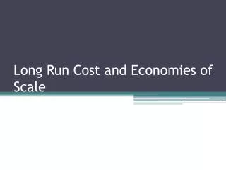
Economies of scale (size) When average cost is falling as output rises, we say the firm experiences economies of scale or increasing returns to size When long run total cost rises proportionately less than output, production is characterized by economies of scale and the LRATC curve slopes downward
AC > MC S > 1 LRAC Economies of Size/Scale MC Long Run Average & Marginal Cost Curves 80 70 60 50 40 30 20 10 0 0 10 20 30 40 y
Why do economies of scale occur? Gains from specialization More efficient use of lumpy inputs blast furnace combine X-ray machine receptionist
Diseconomies of scale (size) When average cost rises as output rises, we say the firm experiences diseconomies of scale or decreasing returns to size When long run total cost rises more than in proportion to output, production is characterized by diseconomies of scale and the LRATC curve slopes upward
AC > MC S > 1 LRAC Diseconomies of Size MC Long Run Average & Marginal Cost Curves 80 70 60 50 40 30 20 10 0 0 10 20 30 40 y
Why do diseconomies of scale occur? Changes in the quality of inputs Supervision and motivation problems Externalities or congestion in production
Constant returns to scale (size) When average cost does not change as output rises, we say the firm experiences constant returns to size or scale When both output and long run total cost rise by the same proportion, production is characterized by constant returns to scale and the LRATC is flat
Why do constant returns to scale occur? Duplication of processes Fixed production proportions and replication Economies and diseconomies balance out
LRAC General shape of the LRAC curve 40 36 32 Cost 28 24 20 16 12 8 4 0 0 5 10 15 20 25 30 Output - y
AC 1 Wagon LAC AC 2 Wagons AC 3 Wagons AC 5 Wagons AC 10 Wagons 0.09 0.08 Cost 0.07 0.06 0.05 0.04 0.03 0.02 0.01 0 500 5500 10500 15500 20500 25500 30500 Output - y