Download
1 / 37
370 likes | 374 Views
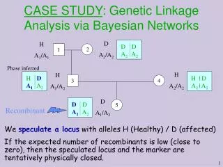
This lecture discusses the use of Bayesian networks for genetic linkage analysis, specifically focusing on recombination and the likelihood function. The lecture also covers the Hidden Markov Model approach and computational tasks involved in the analysis.

E N D
Bayesian network for Recombination L11m L11f L12m L12f X11 S13m X12 S13f y2 y1 L13f L13m X13 y3 L21m L21f L22m L22f X21 S23m X22 S23f L23f L23m X23 is the recombination fraction between loci 2 & 1.
Probability of data (sum over all states of all hidden variables) Prob(data| 2) = P(x11 ,x12 ,x13 ,x21 ,x22 ,x23) = Prob(data| 2) = P(x11 ,x12 ,x13 ,x21 ,x22 ,x23) = l11m, l11f … s23f [P(l11m) P(l11f) P(x11 | l11m, l11f,) … P(s13m) P(s13f) P(s23m |s13m, 2) P(s23m |s13m, 2) ] The likelihood function P(l11m,l11f,x11,l12m,l12f,x12,l13m,l13f,x13, l21m,l21f,x21,l22m,l22f,x22,l23m,l23f,x23, s13m,s13f,s23m,s23f | 2) = Product over all local probability tables = P(l11m) P(l11f) P(x11 | l11m, l11f,) … P(s13m) P(s13f) P(s23m |s13m, 2) P(s23m |s13m, 2) The result is a function of the recombination fraction. The ML estimate is the 2 value that maximizes this function.
Si3f Li2f Xi2 Li2m Li3f Xi3 Li3m Li1f Xi1 Li1m Si3m 2 3 4 1 Locus-by-Locus Summation order Sum over locus i vars before summing over locus i+1 vars Sum over orange vars (Lijt) before summing selector vars (Sijt). This order yields a Hidden Markov Model (HMM).
X1 X1 X2 X2 X3 X3 Xi-1 Xi-1 Xi Xi Xi+1 Xi+1 Recall the resulting HMM S1 S2 S3 Si-1 Si Si+1 X1 X2 X3 Yi-1 Xi Xi+1 The compounded variable Si = (Si,1,m,…,Si,2n,f)is the inheritance vector with 22n states where n is the number of persons that have parents in the pedigree (non-founders). The compounded variable Xi = (Xi,1,m,…,Xi,2n,f) is the data regarding locus i. Similarly for the disease locus we use Yi. To specify the HMM we explicated the transition matrices from Si-1 to Si and the matrices P(xi|Si). Note that these quantities have already been implicitly defined.
Example: Matrix multiplication: versus Multidimensional multiplication/summation: The computational task at hand
Smoking Visit to Asia Tuberculosis Lung Cancer Abnormality in Chest Bronchitis Dyspnea X-Ray An Example • “Asia” network:
S V L T B A X D Compute: • We want to compute P(d) • Need to eliminate: v,s,x,t,l,a,b Initial factors Eliminate: v Note: fv(t) = P(t) In general, result of elimination is not necessarily a probability term
S V L T B A X D Compute: • We want to compute P(d) • Need to eliminate: s,x,t,l,a,b • Initial factors Eliminate: s Summing on s results in a factor with two arguments fs(b,l) In general, result of elimination may be a function of several variables
S V L T B A X D Compute: • We want to compute P(d) • Need to eliminate: x,t,l,a,b • Initial factors Eliminate: x Note: fx(a) = 1 for all values of a !!
S V L T B A X D Compute: • We want to compute P(d) • Need to eliminate: t,l,a,b • Initial factors Eliminate: t
S V L T B A X D Compute: • We want to compute P(d) • Need to eliminate: l,a,b • Initial factors Eliminate: l
S V L T B A X D Compute: • We want to compute P(d) • Need to eliminate: b • Initial factors Eliminate: a,b
Variable Elimination • This process is called variable elimination • Actual computation is done in elimination step • Computation depends on order of elimination
S V L T B A X D Dealing with evidence • How do we deal with evidence? • Suppose get evidence V = t, S = f, D = t • We want to compute P(L, V = t, S = f, D = t)
S V L T B A X D Dealing with Evidence • We start by writing the factors: • Since we know that V = t, we don’t need to eliminate V • Instead, we can replace the factors P(V) and P(T|V) with • These “select” the appropriate parts of the original factors given the evidence • We now continue to eliminate as before.
Complexity of variable elimination Space Complexity is exponential in number of variables in the largest intermediate factor. Or more exactly, space complexity is the size of the largest intermediate factor ) taking into account the number of values of each variable). Time Complexity is the sum of sizes of the intermediate tables.
Some options for improving efficiency • Multiplying special probability matrices efficiently. • Grouping alleles together and removing inconsistent alleles. • Optimizing the elimination order of variables in a Bayesian network. • Performing approximate calculations of the likelihood.
Sometimes conditioning is needed When intermediate tables become too large for a given RAM, even in the optimal order, one can set a value to some indices and iterate. This will decrease the table sizes and trade space with time.
The Constrained Elimination Problem • We define an optimization problem called “The constrained elimination problem”. • The solution of this problem optimizes variable elimination, with or without memory constraints. • We start with the unconstrained version.
Two Operations on a Graph • Eliminating vertex v from a (weighted) undirected graph G – theprocess of making NG(v) a clique and removing v and its incident edges from G. • Conditioning on vertex v in (weighted) undirected graph G – the processof removing vertex v and its incident edges from G. NG(v)is the set of vertices that are adjacent to v in G.
V S L T A B D X V S L T A B D X Example Original Bayes network. • Weights of vertices: • yellow nodes: w = 2 • blue nodes: w = 4 Undirected graph representation. P(v,s,…,x)= p(v) p(s) p(t|v) p(l|s)p(a|t,l)p(b|l)
The residual graph Gi is the graph obtained from Gi-1 by • eliminating vertex Xα(i-1). (G1≡G). • The cost of an elimination sequence Xα is the sum of • costs of eliminating Xα(i) from Gi, for all i. Elimination Sequence • Elimination sequence of G – an order of the vertices of G, writtenasXα= (Xα(1) ,…,Xα(n) ),where αis a permutation on {1,…,n}. • The cost of eliminating vertex v from a graph Gi is the • product of weights of the vertices in NGi(v).
G2 G3 G1 S S V S L L L T T T A B A A B D D D X X X Example Suppose the elimination sequence is Xα=(V,B,S,…):
Relation to Treewidth • The unconstrained Elimination Problem reduces to finding treewidth if: • the weight of each vertex is constant, • the cost function is • Finding the treewidth of a graph is known to be NP-complete (Arnborg et al., 1987). • When no edges are added, the elimination sequence is perfect and the graph is chordal. • Optimal elimination sequence: one with • minimal cost.
Constrained elimination sequence • Xα,β =((Xα(1),…,,Xα(n)),β), whereβis a binary • vector of length n, such that: Constrained Elimination Sequence Optimal constrained elimination sequences yield optimal variable elimination under memory constraints.
G2 G3 G1 S S V S L L L T T T A B A A B D D D X X X Example Suppose the constrained elimination sequence is Xα,β=((V,B,S,…),(0,1,0,…)):
Cost of a Constrained Elimination Sequence • The elimination cost of a constrained elimination sequence Xα,βis:
The Constrained Elimination Problem • Input: G(V,E,w), threshold T. • Find a constrained elimination sequenceXα,β which satisfies: • Its elimination cost is minimal. • The elimination cost of eachXα(i)is lower than T.
Deterministic Greedy Algorithm • Iteration i: a vertex Xi is chosen whose elimination cost is minimal. • If the elimination cost of every vertex in Gi is above T, then a vertex Xi is chosen to be fixed (instead of eliminated). ni(X) is the number of cliques in Gi that include X.
Stochastic Greedy Algorithm • Iteration i: Three variables with minimal elimination cost are found and a coin is flipped to choose between them. The coin is biased according to the elimination costs of the vertices. • If the elimination cost of every vertex in Gi is above T, then a vertex Xi is chosen to be fixed (instead of eliminated). • Repeat many times (say, 100) unless the cost becomes low.
Standard usage of linkage There are usually 5-15 markers. 20-30% of the persons in large pedigrees are genotyped (namely, their xij is measured). For each genotyped person about 90% of the loci are measured correctly. Recombination fraction between every two loci is known from previous studies (available genetic maps). The user adds a locus called the “disease locus” and places it between two markers i and i+1. The recombination fraction ’between the disease locus and marker i and ” between the disease locus and marker i+1 are the unknown parameters being estimated using the likelihood function. This computation is done for every gap between the given markers on the map. The MLE hints on the whereabouts of a single gene causing the disease (if a single one exists).
SUPERLINK • Stage 1: each pedigree is translated into a Bayesian network. • Stage 2: value elimination is performed on each pedigree (i.e., some of the impossible values of the variables of the network are eliminated). • Stage 3: an elimination order for the variables is determined, according to some heuristic. • Stage 4: the likelihood of the pedigrees given the values is calculated using variable elimination according to the elimination order determined in stage 3. • Allele recording and special matrix multiplication is used.
over 100 hours Out-of-memory Pedigree size Too big for Genehunter. Experiment A (V1.0) • Same topology (57 people, no loops) • Increasing number of loci (each one with 4-5 alleles) • Run time is in seconds.
Vitesse doesn’t handle looped Pedigrees. Out-of-memory Pedigree size Too big for Genehunter. Experiment B (V1.0) • Same topology (100 people, with loops) • Increasing number of loci (each one with 5-10 alleles) • Run time is in seconds.
Bus error Out-of-memory Experiment C (V1.0) • Same topology (5 people, no loops) • Increasing number of loci (each one with 3-6 alleles) • Run time is in seconds.