Download
1 / 43
430 likes | 523 Views
Trees (Ch. 10.2) Longin Jan Latecki Temple University based on slides by Simon Langley, Shang-Hua Teng, and William Albritton. Section 10.2: Applications of Trees. Binary search trees A simple data structure for sorted lists Decision trees Minimum comparisons in sorting algorithms

E N D
Trees (Ch. 10.2)Longin Jan LateckiTemple Universitybased on slides bySimon Langley, Shang-Hua Teng, and William Albritton
Section 10.2: Applications of Trees • Binary search trees • A simple data structure for sorted lists • Decision trees • Minimum comparisons in sorting algorithms • Prefix codes • Huffman coding
Basic Data Structures - Trees • Informal: a tree is a structure that looks like a real tree (up-side-down) • Formal: a tree is a connected graph with no cycles.
Trees - Terminology size=7 root subtree x value b e m height=2 c d a nodes leaf Every node must have its value(s) Non-leaf node has subtree(s) Non-root node has a single parent node
Types of Tree Binary Tree Each node has at most 2 sub-trees m-ary Trees Each node has at most m sub-trees
Binary Search Trees A binary search tree: • … is a binary tree. • if a node has value N, all values in its left sub-tree are less than or equal to N, and all values in its right sub-tree are greater than N.
Binary Search Tree Format Example: • Items are stored at individual tree nodes. • We arrange for the tree to always obey this invariant: • For every item x, • Every node in x’s left subtree is less than x. • Every node in x’s right subtree is greater than x. 7 3 12 1 5 9 15 0 2 8 11
Searching a binary search tree Time per level search(t, s) { If(s == label(t)) return t; If(t is leaf) return null If(s < label(t)) search(t’s left tree, s) else search(t’s right tree, s)} O(1) O(1) h Total O(h)
Searching a binary search tree Time per level search( t, s ) { while(t != null) { if(s == label(t)) return t; if(s < label(t) t = leftSubTree(t); else t = rightSubTree(t); } return null; O(1) O(1) h Total O(h)
Here’s another function that does the same (we search for label s): TreeSearch(t, s) while (t != NULL and s != label[t]) if (s < label[t]) t = left[t]; else t = right[t]; return t;
Insertion in a binary search tree:we need to search before we insert Insert 6 Insert 11 6 11 6 11 6 6 11 always insert to a leaf ? Time complexity O(height_of_tree) n = size of the tree O(log n) if it is balanced
Insertion insertInOrder(t, s) { if(t is an empty tree) // insert here return a new tree node with value s else if( s < label(t)) t.left = insertInOrder(t.left, s ) else t.right = insertInOrder(t.right, s) return t }
Recursive Binary Tree Insert procedure insert(T: binary tree, x: item)v := root[T]if v = null then begin root[T] := x; return “Done” endelse if v = xreturn “Already present”else if x < vthenreturn insert(leftSubtree[T], x)else{must be x > v}return insert(rightSubtree[T], x)
Comparison –Insertion in an ordered list insertInOrder(list, s) { loop1: search from beginning of list, look for an item >= s loop2: shift remaining list to its right, start from the end of list insert s } Insert 6 6 6 6 6 8 9 6 2 3 4 5 7 6 7 8 9 Time complexity? O(n) n = size of the list
Try it!! • Build binary search trees for the following input sequences • 7, 4, 2, 6, 1, 3, 5, 7 • 7, 1, 2, 3, 4, 5, 6, 7 • 7, 4, 2, 1, 7, 3, 6, 5 • 1, 2, 3, 4, 5, 6, 7, 8 • 8, 7, 6, 5, 4, 3, 2, 1
Decision Trees • A decision tree represents a decision-making process. • Each possible “decision point” or situation is represented by a node. • Each possible choice that could be made at that decision point is represented by an edge to a child node. • In the extended decision trees used in decision analysis, we also include nodes that represent random events and their outcomes.
Coin-Weighing Problem • Imagine you have 8 coins, oneof which is a lighter counterfeit, and a free-beam balance. • No scale of weight markings is required for this problem! • How many weighings are needed to guarantee that the counterfeit coin will be found? ?
As a Decision-Tree Problem • In each situation, we pick two disjoint and equal-size subsets of coins to put on the scale. A given sequence ofweighings thus yieldsa decision tree withbranching factor 3. The balance then“decides” whether to tip left, tip right, or stay balanced.
Applying the Tree Height Theorem • The decision tree must have at least 8 leaf nodes, since there are 8 possible outcomes. • In terms of which coin is the counterfeit one. • Recall the tree-height theorem, h≥logm. • Thus the decision tree must have heighth≥ log38 = 1.893… = 2. • Let’s see if we solve the problem with only 2 weightings…
General Solution Strategy • The problem is an example of searching for 1 unique particular item, from among a list of n otherwise identical items. • Somewhat analogous to the adage of “searching for a needle in haystack.” • Armed with our balance, we can attack the problem using a divide-and-conquer strategy, like what’s done in binary search. • We want to narrow down the set of possible locations where the desired item (coin) could be found down from n to just 1, in a logarithmic fashion. • Each weighing has 3 possible outcomes. • Thus, we should use it to partition the search space into 3 pieces that are as close to equal-sized as possible. • This strategy will lead to the minimum possible worst-case number of weighings required.
Coin Balancing Decision Tree • Here’s what the tree looks like in our case: 123 vs 456 left: 123 balanced:78 right: 456 4 vs. 5 1 vs. 2 7 vs. 8 L:1 L:4 L:7 R:2 B:3 R:5 B:6 R:8
General Balance Strategy • On each step, putn/3of the n coins to be searched on each side of the scale. • If the scale tips to the left, then: • The lightweight fake is in the right set ofn/3≈ n/3 coins. • If the scale tips to the right, then: • The lightweight fake is in the left set of n/3≈ n/3coins. • If the scale stays balanced, then: • The fake is in the remaining set ofn− 2n/3 ≈ n/3coins that were not weighed! You can prove that this strategy always leads to a balanced 3-ary tree.
Data Compression • Suppose we have 3GB character data file that we wish to include in an email. • Suppose file only contains 26 letters {a,…,z}. • Suppose each letter a in {a,…,z} occurs with frequency fa. • Suppose we encode each letter by a binary code • If we use a fixed length code, we need 5 bits for each character • The resulting message length is • Can we do better?
Data Compression: A Smaller Example • Suppose the file only has 6 letters {a,b,c,d,e,f} with frequencies • Fixed length 3G=3000000000 bits • Variable length Fixed length Variable length
How to decode? • At first it is not obvious how decoding will happen, but this is possible if we use prefix codes
Prefix Codes • No encoding of a character can be the prefix of the longer encoding of another character: • We could not encode t as 01 and x as 01101 since 01 is a prefix of 01101 • By using a binary tree representation we generate prefix codes with letters as leaves
Decoding prefix codes • Follow the tree until it reaches to a leaf, and then repeat! • A message can be decoded uniquely!
Prefix codes allow easy decoding Decode: 11111011100 s 1011100 sa 11100 san 0 sane
Some Properties • Prefix codes allow easy decoding • An optimal code must be a full binary tree (a tree where every internal node has two children) • For C leaves there are C-1 internal nodes • The number of bits to encode a file is where f(c) is the freq of c, lengthT(c) is the tree depth of c, which corresponds to the code length of c
Optimal Prefix Coding Problem • Given is a set of n letters (c1,…, cn) with frequencies (f1,…, fn). • Construct a full binary tree T to define a prefix code that minimizes the average code length
Greedy Algorithms • Many optimization problems can be solved using a greedy approach • The basic principle is that local optimal decisions may be used to build an optimal solution • But the greedy approach may not always lead to an optimal solution overall for all problems • The key is knowing which problems will work with this approach and which will not • We study • The problem of generating Huffman codes
Greedy algorithms • A greedy algorithm always makes the choice that looks best at the moment • My everyday examples: • Driving in Los Angeles, NY, or Boston for that matter • Playing cards • Invest on stocks • Choose a university • The hope: a locally optimal choice will lead to a globally optimal solution • For some problems, it works • Greedy algorithms tend to be easier to code
David Huffman’s idea • A Term paper at MIT • Build the tree (code) bottom-up in a greedy fashion Each tree has a weight in its root and symbols as its leaves. We start with a forest of one vertex trees representing the input symbols. We recursively merge two trees whose sum of weights is minimal until we have only one tree.
The Huffman Coding algorithm- History • In 1951, David Huffman and his MIT information theory classmates given the choice of a term paper or a final exam • Huffman hit upon the idea of using a frequency-sorted binary tree and quickly proved this method the most efficient. • In doing so, the student outdid his professor, who had worked with information theory inventor Claude Shannon to develop a similar code. • Huffman built the tree from the bottom up instead of from the top down
Huffman Coding Algorithm • Take the two least probable symbols in the alphabet • Combine these two symbols into a single symbol, and repeat.
1.0 0 0.55 1 1 0 0.45 0.3 0 1 0 1 Example • Ax={ a , b , c , d , e } • Px={0.25, 0.25, 0.2, 0.15, 0.15} a 0.25 c 0.2 d 0.15 b 0.25 e 0.15 00 10 11 010 011
Building the Encoding Tree Building the Encoding Tree
Building the Encoding Tree Building the Encoding Tree
Building the Encoding Tree Building the Encoding Tree