Download
1 / 42
460 likes | 727 Views
ECMWF Data Assimilation Training Course - Kalman Filter Techniques. Mike Fisher. Kalman Filter – Derivation. Consider a general linear analysis: where y is a vector of observations, x b is a background. K and L are matrices.

E N D
ECMWFData AssimilationTraining Course -Kalman Filter Techniques Mike Fisher
Kalman Filter – Derivation • Consider a general linear analysis: • where y is a vector of observations, xb is a background. K and L are matrices. • Suppose also that we have an operator H that takes us from model space to observation space. • Assume this can be done without error, so that: • We require that, if y and xb are error-free, the analysis should also be error-free: • I.e.
Kalman Filter – Derivation • Consider any analysis of the form: • Define errors, • Then: • Where is representativeness error. • ( is often ignored.) • Assume that the errors are unbiased.
Kalman Filter – Derivation • Assume that is uncorrelated with • The covariance matrix for the analysis error is:
Kalman Filter – Derivation • Use the following matrix calculus identities: • To get:
Kalman Filter – Derivation • Minimum variance => • I.e. • This is the Kalman gain matrix
Kalman Filter – Derivation • The Kalman filter consists of two sets of equations. • The first set define the minimum–variance, linear analysis, and its covariance matrix: • where:
Kalman Filter – Derivation • The second set of equations describe how to propagate the state and the covariance matrix so that they can be used for the background for the next cycle of analysis. • For the state, we have: • where is a linear model. • The equation for the error is: • where is the model error.
Kalman Filter – Derivation • Assume that model error is unbiased, and uncorrelated with analysis error, and form the covariance matrix: • I.e.
Kalman Filter – Derivation • The Kalman Filter Equations:
Extended Kalman Filter (EKF) • The Extended Kalman Filter is an ad hoc generalization of the Kalman filter to weakly non-linear systems. • The forecast model and observation operators are allowed to be non-linear: • The matrices and in the equations for and are the linearized about and . • NB: The EKF requires tangent linear and adjoint codes! • The Iterated Extended Kalman Filter (IEKF) repeats the linearization of Hk as soon as a better estimate for the state is available – much like incremental 4dVar.
Kalman Filter for Large Dimensions • The Kalman filter is impractical for large dimension systems. • It requires us to handle matrices of dimension N×N, where N is the dimension of the state vector. • This is out of the question if N~106. • Propagating the covariance matrix using: requires N integrations of the tangent linear model. • Even the matrix multiplies required to construct are prohibitively expensive. • A range of reduced-rank, approximate Kalman filters have been developed for use in large systems.
Reduced-Rank Methods • Reduced-rank methods approximate the Kalman filter by restricting the covariance equations to a small subspace. • Suppose we can write , where is N×K, with K small (e.g. K~100). • The Kalman gain becomes : • The initial in this equation means that the analysis error covariance is also restricted to the subspace:
Reduced-Rank Methods • Hence, the covariance may be propagated using only K integrations of the linear model: • We can then project onto a new subspace to generate an approximate covariance matrix for use in the next analysis cycle.
Reduced-Rank Methods • It is important to remember that reduced-rank Kalman filters are approximations to the full Kalman filter. • They are not optimal. • How sub-optimal are they, e.g. compared to 4dVar? • The jury is still out! • A particular defect is the leading in: • This means that the analysis increment is restricted to lie in the space spanned by the columns of . • This is sometimes called the “rank problem”.
Reduced-Rank Methods • Another consequence of approximating by a low-rank matrix is that spurious long-range correlations are produced. • Example: • Suppose there is a spurious long-range correlation between Antarctica and Europe. • The analysis will find it difficult to generate increments over Antarctica, since these will contradict the observations over Europe. • More generally, the analysis will not have enough available degrees of freedom to allow it to fit all the observations (100 degrees of freedom v. 105 obs!). • Two ways around this problem are: • Local analysis (e.g. Evensen, 2003, Ocean Dynamics pp 343-367) • Schur product (e.g. Houtekamer and Mitchell, 2001, MWR pp123-137)
Ways Around the Rank Problem • Local analysis solves the analysis equations independently for each gridpoint (or for each of a set of regions). • Each analysis uses only observations that are local to the gridpoint (or region). • In this way, the analysis at each gridpoint (or region) is not influenced by distant observations. • The global analysis is no longer a linear combination of the spanning vectors. • The method acts to vastly increase the effective rank of the covariance matrix. • The analysis is sub-optimal because, at each gridpoint, only a subset of available information is used.
Ways Around the Rank Problem • The Schur product of two matrices, denoted , is the element-wise product: . • Spurious, long-range correlations may be removed from by forming the Schur product of the covariance matrix with a matrix representing a decaying function of distance. • The modified covariance matrix is never explicitly formed (it is too big). Rather, the method deals with terms such as . • The Schur product also has the effect of vastly increasing the effective rank of the covariance matrix. • Choosing the product function is non-trivial. It is easy to modify the correlations in undesirable ways. E.g. balance relationships may be adversely affected.
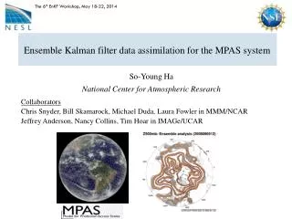
Ensemble Methods • Ensemble Kalman filters are reduced-rank Kalman filters that construct their covariance matrices as sample covariance matrices: • where the index, i, refers to sample (ensemble) member. • is a sample (ensemble) of background states whose sample covariance matrix is an estimate of the true background error covariance matrix.
Ensemble Methods • The terms involving in the analysis equation are represented as sample error covariance matrices: • It is never necessary to explicitly form the N×N background error covariance matrix. • No tangent linear or adjoint observation operators or models are required.
Ensemble Methods • The sample of background states is generated from a sample of analysis states, : • where is a noise process with covariance matrix Qk+1. • NB: The full nonlinear model is used to propagate the states. • The random sample , may be generated by perturbing the observations with random noise drawn from the covariance matrix of observation error (Burgers et al., 1998, MWR pp 1719-1724). • This method is similar to the analysis-ensemble method for generating Jb statistics.
Ensemble Methods • Adding noise to the observations results in a small amount of additional sampling noise. • This additional noise is avoided in the Ensemble Adjustment Kalman Filter (EAKF, Anderson 2001, MWR 2884-2903) and the Ensemble Transform Kalman Filter (ETKF, Bishop et al. 2001, MWR 420-436).
Ensemble Methods • The ensemble adjustment Kalman filter avoids the need to add noise by implicitly calculating a matrix A, such that: • and • The ensemble transform Kalman filter calculates T such that Va represents an analysis sample in: • These methods can be more accurate than the perturbed-observation method, but they make heavier demands on the linearity of the underlying system, and on the Gaussian assumption for the statistics.
Other Low-Rank Methods • Ensemble methods are popular and attractive because they don’t require adjoint or tangent linear codes. However, a random basis is unlikely to be optimal. • Singular vectors, bred modes, etc. can be used to define deterministic subspaces for reduced-rank Kalman filtering that attempt to capture important aspects of covariance evolution. • ECMWF RRKF (R.I.P.) • defined a subspace that evolved into the leading eigenvectors of the forecast error covariance matrix at day 2. • SEEK, SEIK, SSEIK, SEPLK (Pham et al, 1998) • a plethora of evolving/partially-evolving subspaces and a plague of acronyms! • Reduced Order Kalman Filter (Farrell and Ioannou, 2001) • uses model-reduction techniques to define an optimal subspace.
Non-Gaussian Methods • Particle filters approximate the forecast pdf by a discrete distribution: • An ensemble of forecasts, x(1)...x(K) is run. Each member of the ensemble has an associated weight, w(i). • When an observation is available, the weights are adjusted using Bayes’ theorem. E.g: • Eventually, the weights for some members become tiny. • These members are dropped from the ensemble, and replaced by new, more probable members.
Non-Gaussian Methods • Particle filters work well for highly-nonlinear, low-dimensional systems. • Successful applications include missile tracking, computer vision, etc. (see the book “Sequential Monte Carlo Methods in Practice”, Doucet, de Freitas, Gordon (eds.), 2001) • van Leeuwen (2003) has successfully applied the technique for an ocean model. • The main problem to be overcome is that, for a large-dimensional system, with lots of observations, almost any forecast will contradict an observation somewhere on the globe. • => Every cycle, unless the ensemble is truly enormous, all the particles (forecasts) are highly unlikely (given the obseravtions). • van Leeuwen has recently suggested methods that may get around this problem.
Non-Gaussian Methods Estimated initial location of robot Where am I? Actual initial location of robot from: Fox et al. 1999, proc 16th National Conference on Artificial Intelligence
Non-Gaussian Methods from: Fox et al. 1999, proc 16th National Conference on Artificial Intelligence
The Non-Sequential Approach • All the preceding is based on the sequential (recursive) view of the filtering problem: • An optimal estimate for step k+1 is produced using only the state and covariance matrices from step k. • All the information from earlier steps is brought to the present step via the covariance matrices. • The advantage of the sequential approach is that we don’t need to go back any further than the previous step in order to determine the current analysis. • The disadvantage is that we must explicitly propagate the covariance matrices. • For very large systems, the matrices are so enormous that a non-sequential approach may be preferable.
Equivalence of Kalman Smoother and 4dVar • Suppose we want to produce the optimal estimate of the states x0...xK, at steps 0...K, given observations y0...yK at steps 0...K, and a background state xb at step 0. • Assuming errors are Gaussian, the probability of x0...xK given y0...yK and xb is:
Equivalence of Kalman Smoother and 4dVar • Taking the logarithm gives us the weak-constraint 4dVar cost function: • The maximum likelihood solution is given by the minimum of the cost function. • For Gaussians, this is also the minimum-variance solution. • Hence, at step K, weak-constraint 4dVar gives the same (minimum-variance) solution as the Kalman filter.
Equivalence of Kalman Smoother and 4D-Var • The solution of the minimization problem differs from the Kalman filter solution at steps 0…K-1. • The 4dVar solution for step k is optimal with respect to observations at steps 0…K. • The Kalman filter solution at step k is optimal only with respect to observations at steps 0…k. • I.e. weak constraint 4D-Var is equivalent to the Kalman smoother. • A purely algebraic proof of this equivalence is given by Ménard and Daley (1996, Tellus 48A, 221-237). (See also Li and Navon (2001) QJRMS, 661-684.) • This proof shows that the equivalence does not depend on the statistical assumptions made in formulating the analysis problem.
The Non-Sequential Approach • So, to determine the optimal state at step K, given observations at steps 0...K, and a background at step 0, we can: • Either: run a sequential Kalman filter, starting from the background at step 0, and updating the N×N covariance matrices at each step. • Or: minimize the weak-constraint 4dVar cost function using all observations for steps 0…K. • The sequential approach is impractical for large N. • In principle, the 4dVar approach becomes impractical as K becomes large. • What may save 4dVar is the limited memory of the Kalman filter. • The analysis is insensitive to observations in the distant past • => We can minimize over steps K-p...K, instead of 0...K.
Martin Leutbecher’s “Planet L95” EKF (Lorenz, 1995, ECMWF Seminar on Predictability, and Lorenz and Emanuel, 1998) unit time ~ 5 days Chaotic system: 13 positive Lyapunov exponents. The largest exponent corresponds to a doubling time of 2.1 days.
analysis fc analysis Demonstration of Long-Window 4dVar for the L95 Toy Problem • Weak-constraint 4dVar was run for 230 days, with window lengths of 1-10 days. • One cycle of analysis performed every 6 hours. • NB: Analysis windows overlap. • Obs every 6h at 3 out of every 5 grid-points. • First guess was constructed from the overlapping part of the preceding cycle, plus a 6-hour forecast: • Quadratic cost function! • No background term in the cost function!
Mean RMS Analysis Error RMS error at end of 4dVar window. NB: No background term! RMS error for OI RMS error for EKF
Analysis experiments started with/without satellite data on 1st August 2002 More Evidence Memory of the initial state disappears after approx. 7 days from: Graeme Kelly
Analysis experiment started with satellite data reintroduced on 16th August 2005 Limited Memory Memory of the initial state disappears after approx. 3 days
Analysis experiment started with satellite data reintroduced on 16th August 2005 Limited Memory Memory of the initial state disappears after approx. 3 days
Long-Window, Weak-Constraint 4dVar • Long window, weak constraint 4dVar is equivalent to the Kalman filter, provided we make the window long enough. • For NWP, 3-10 days is long enough. • Long-window, weak constraint 4dVar is feasible (but expensive). • The resulting Kalman filter is full-rank.
Summary • The Kalman filter is the optimal (minimum-variance) analysis for a linear system. • For weakly nonlinear systems, the extended Kalman filter can be used, but it needs adjoints and tangent linear models and observation operators. • Ensemble methods are relatively easy to develop (no adjoints required), but little rigorous investigation of how well they approximate a full-rank Kalman filter has been carried out. • Particle filters are interesting, but it is not clear how useful they are for large-dimension systems. • For large systems, the covariance matrices are too big to be handled. • We must either use low-rank approximations of the matrices (and risk destroying the advantages of the Kalman filter) • Or use the non-sequential approach (weak-constraint 4dVar).