Download
1 / 54
540 likes | 719 Views
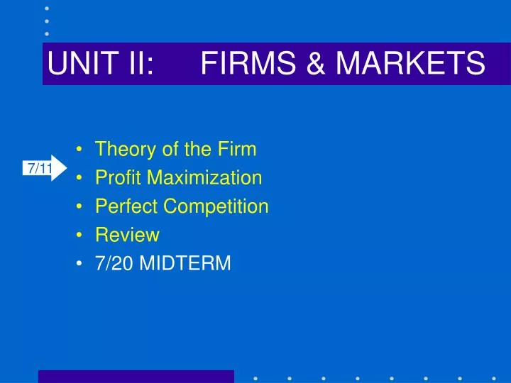
UNIT II: FIRMS & MARKETS. Theory of the Firm Profit Maximization Perfect Competition Review 7 /20 MIDTERM. 7/11. Theory of the Firm. Cost Minimization The Short-Run and the Long- Run Profit Maximization Firm and Market Supply Perfect Competition (Part 1). Cost Minimization.

E N D
UNIT II: FIRMS & MARKETS • Theory of the Firm • Profit Maximization • Perfect Competition • Review • 7/20 MIDTERM 7/11
Theory of the Firm • Cost Minimization • The Short-Run and the Long-Run • Profit Maximization • Firm and Market Supply • Perfect Competition (Part 1)
Cost Minimization Consider a firm that produces output according to the following production function: Q = 4K½L½ Assume that w = $18 and r = $36, and the firm currently has 16 units of capital. With K = 16, the firm’s short-run production function is: Q = 16L½ For Q = 10, 10 = 16L½ => L = 100/256 = .39
Cost Minimization Consider a firm that produces output according to the following production function: Q = 4K½L½ Assume that w = $18 and r = $36, and the firm currently has 16 units of capital. To produce 10 units: 10 = 16L½ => L = 100/256 =.39 With K = 16, the firm’s total cost of production is: TC = rK + wL = 36(16) + 18(.39) = $583.03
Cost Minimization Consider a firm that produces output according to the following production function: Q = 4K½L½ Assume that w = $18 and r = $36, and the firm currently has 16 units of capital. More generally: Q = 16L½ => L = (Q/16)2 With K = 16, the firm’s short-run total cost function is: TC = rK + wL = 36(16) + 18(Q/16)2 = $576 + 18(Q/16)2
Cost Minimization in the Short-Run How much will it cost this firm to produce Q units of output in the short-run? Total Cost Function TCsr = 576 + 18(Q/16)2 $ Fixed Costs = rK = 36(16) = $576 Q
Cost Minimization in the Short-Run How much will it cost this firm to produce 10 units of output in the short-run? In the short-run,if the firm wants to produce more (or less) than 10 units, it would move along it’s short-run output-expansionpath, at K =16. K K = 16 Q = 10 L = 0.39 L
Cost Minimization in the Long-Run How much will it cost this firm to produce 10 units of output in the long-run? In the long-run, all factors are variable. Firms combine factors of production in a manner analogous to the way consumers choose a consumption bundle. K Q = 10 L
Cost Minimization in the Long-Run How much will it cost this firm to produce 10 units of output in the long-run? An isoquant is all the technologically efficient combinations of K ,L to produce a certain output, Q. K Isoquant Slope = - MRTS Q = 10 L
Cost Minimization in the Long-Run How much will it cost this firm to produce 10 units of output in the long-run? If we think of the allthe combinations of K&L that cost a certain amount (TC), we have anisocost line: K = TC/r – (w/r)L Recall: TC = wL + rK K Isocost lines Slope = - w/r Q = 10 L
Cost Minimization in the Long-Run How much will it cost this firm to produce 10 units of output in the long-run? Tangency between the isoquant and an isocost curve shows the economically efficient combination K*, L*. Hence, the condition for optimal factor proportion is: MRTS = w/r K K* Isocost lines Slope = - w/r Isoquant Slope = - MRTS Q = 10 L* L
Cost Minimization in the Long-Run How much will it cost this firm to produce 10 units of output in the long-run? The condition for optimal factor proportion is: MRTS = w/r This is LR condition!Why? Because some factors (K) are fixed in the SR. K K* Isocost lines Slope = - w/r Isoquant Slope = - MRTS Q = 10 L* L
Cost Minimization in the Long-Run How much will it cost this firm to produce 10 units of output in the long-run? Another way to think about this: TC is a projection of the firm’s long-run output expansion path: the locus of optimal factor bundles (K,L) for different levels of Q. (Constant return depicted) K K* Q = 10 L* L
Cost Minimization in the Long-Run How much will it cost this firm to produce 10 units of output in the long-run? To find total cost in terms of Q, we use the cost minimization condition and the production function to find substitute expressions in terms of Q for K and L. Cost minimization requires that the firm produce using a combination of inputs for which the ratios of the marginal products, or the marginal rate of technical substitution, equals the ratio of the input prices: MRTS = w/r
Cost Minimization in the Long-Run How much will it cost this firm to produce 10 units of output in the long-run? Q = 4K1/2L1/2 w = 18; r = 36 MRTS = MPL/MPK MPL = 2K1/2L-1/2 MPK = 2K-1/2L1/2 MRTS = K/L. = w/r = 18/36 = L = 2K. The firm’s optimal factor proportion (given technology and factor prices).
Cost Minimization in the Long-Run How much will it cost this firm to produce 10 units of output in the long-run? Q = 4K1/2L1/2 L = 2K => Q = 4K1/2(2K)1/2 = 4(2)1/2K Q = 4(2)1/2K => K = Q/[4(2)1/2] Q = 5.66K => K = Q/5.66 For Q =10 => K = 1.77; L = 3.54 TC = wL + rK TC(Q=10) = 36(1.77)+18(3.54) = $127.28 To produce 10 units of output, we solve for K and L in terms of Q and substitute in the total cost function. Producing 10 units costs $127.28. At this point, the firm is using 1.77 units of capital and 3.54 units of labor.
Cost Minimization in the Long-Run How much will it cost this firm to produce 10 units of output in the long-run? Q = 4K1/2L1/2 L = 2K => Q = 4K1/2(2K)1/2 = 4(2)1/2K Q = 4(2)1/2K => K = Q/[4(2)1/2] Q = 5.66K => K = Q/5.66 For Q =10 => K = 1.77; L = 3.54 TC = wL + rK TC(Q=10) = 36(1.77)+18(3.54) = $127.28 Comparing this to the short-run, the cost of production is lower in the long-run, because the firm is now able to adjust K as well as L to minimize the cost of the production of a given amount of output, which is more efficient.
Cost Minimization in the Long-Run How much will it cost this firm to produce Q units of output in the long-run? TC = 18L + 36K = 9Q/(2)1/2 + 9Q/(2)1/2 = 18/(2)1/2(Q) = 12.73Q MC = 12.73 = AC We can also solve for the firm’slong run total cost function for any level of output. . The long-run total cost curve (TC(Q)) represents the minimum cost to produce Q units of output.
Cost Minimization in the Long-Run Graphically: Q = 4K1/2L1/2 w = 18; r = 36 TCsr = 576 + 18(Q/16)2 $ TClr = 12.73Q MC = 12.73 Fixed Costs = rK = $576 Q
Cost Minimization We have seen that we can solve the firm’s cost minimization problem analogously to the consumer’s utility maximization problem. Cost minimization requires that the firm produce using a combination of inputs for which the ratios of the marginal products, or the marginal rate of technical substitution, equals the ratio of the input prices: MRTS = w/r • 2 Provisos: • Only in the Long-Run • Only part of the firm’s problem
Cost Minimization in the Long-Run How much will it cost this firm to produce 10 units of output in the long-run? Q = 4K1/2L1/2 w = 18; r = 36 MRTS = MPL/MPK MPL = 2K1/2L-1/2 MPK = 2K-1/2L1/2 MRTS = K/L. = w/r = 18/36 = L = 2K. The firm’s optimal factor proportion (given technology and factor prices).
Cost Minimization in the Long-Run How much will it cost this firm to produce 10 units of output in the long-run? L = 2K Tangency between the isoquant and an isocost curve shows the economically efficient combination K*, L*. Hence, the condition for optimal factor proportion is: MRTS = w/r K K* Q = 10 L* L
Cost Minimization in the Long-Run How much will it cost this firm to produce 10 units of output in the long-run? L = 2K The condition for optimal factor proportion is: MRTS = w/r This is LR condition!Why? Because some factors (K) are fixed in the SR. K K* Q = 10 L* L
Cost Minimization in the Long-Run How much will it cost this firm to produce Q units of output in the long-run? L = 2K Another way to think about this: TC is a projection of the firm’s long-run output expansion path: the locus of optimal factor bundles (K,L) for different levels of Q. K K* Q = 10 L* L
Cost Minimization in the Long-Run How much will it cost this firm to produce Q units of output in the long-run? TC(Q) = 18L + 36K = 9Q/(2)1/2 + 9Q/(2)1/2 = 18/(2)1/2(Q) = 12.73Q MC(Q) = 12.73 = AC(Q) K K* We can solve for the firm’slong run total cost function for any level of output. Q = 10
Cost Minimization Graphically: Q = 4K1/2L1/2 w = 18; r = 36 In the SR, K = 16 TCsr = 576 + 18(Q/16)2 $ TClr = 12.73Q At this point, 16 units of capital is optimal. MC = 12.73 Fixed Costs = rK = $576 Q
Profit Maximization Profit (P) = Total Revenue(TR) – Total Cost(TC) $ Consider a firm with long-run total costs TC. TC Q1 Q2 Q3 Q
Profit Maximization Profit (P) = Total Revenue(TR) – Total Cost(TC) $ To maximize profits, the firms finds Q where distance between TC and TR is greatest. the same slope. TR = PQ TC Q1 Q2 Q3 Q
Profit Maximization Profit (P) = Total Revenue(TR) – Total Cost(TC) $ To maximize profits, the firms finds Q where distance between TC and TR is greatest.same slope. TC TR = PQ Q1 Q2 Q3 Q
Profit Maximization Profit (P) = Total Revenue(TR) – Total Cost(TC) $ To maximize profits, the firms finds Q where distance between TC and TR is greatest.same slope. TC TR = PQ Q1 Q2 Q3 Q
Profit Maximization Profit (P) = Total Revenue(TR) – Total Cost(TC) $ To maximize profits, the firm finds Q where distance between TC and TR is greatest. This will be where they have the same slope.. slope. TR = PQ Pmax TC Q1 Q2 Q3 Q* Q
Profit Maximization Marginal Analysis: If TC is rising faster than TR, reduce Q. If TR is rising faster than TC, increase Q. Profit (P) = Total Revenue(TR) – Total Cost(TC) $ TR = PQ Pmax TC Q1 Q2 Q3 Q* Q
Profit Maximization Marginal Analysis: Recall: slope TR = MR slope TC = MC Hence, to maximize profits: MR = MC Profit (P) = Total Revenue(TR) – Total Cost(TC) $ TR = PQ Pmax TC Q1 Q2 Q3 Q* Q
Profit Maximization The firm wants to maximize this difference: Profit (P) = Total Revenue(TR) – Total Cost(TC) TR(Q) = PQ TC(Q) = rK + wL P Price L Labor Q Quantity K Capital w Wage Rate r Rate on Capital Q = f(K,L) Revenue Cost
Profit Maximization Demand for the firm’s output is given by Q = 100 – 2P. Find the firm’s profit maximizing level of output. Q = 4K1/2L1/2 w = 18; r = 36 Q = 100 – 2P => P = 50 – 1/2Q TR = PQ = (50 – 1/2Q)Q = 50Q – 1/2 Q2 MR = 50 – Q = MC = 12.73 => Q* = 37.27; P* = 31.37
Profit Maximization Demand for the firm’s output is given by Q = 100 – 2P. Find the firm’s profit maximizing level of output. Q = 4K1/2L1/2 w = 18; r = 36 Q = 100 – 2P => P = 50 – 1/2Q TR = PQ = (50 – 1/2Q)Q P = TR – TC = 50Q – 1/2 Q2 – 12.73Q FOC: dP/dQ = 50 – Q – 12.73 = 0 => Q* = 37.27; P* = 31.37
Profit Maximization in the Long-Run We solved the firm’s optimization problem focusing on the profit output level, Q*, but it is important to emphasize that the optimization principle also tell us about input choices. When the firm chooses an output level Q* that maximizes P for given factor prices (w, r), the firm has simultaneously solved for L* and K*. To produce Q* = 37.27 (given the production function, Q = 4K1/2L1/2, and optimal factor proportion, L = 2K), we find: L* = 6.58; K* = 3.29. Finally, P = TR–TC = PQ–12.73Q = (31.37–12.73)37.27 = $694.71.
Profit Maximization in the Short-Run We saw that the firm maximizes profit by choosing a level of output such that marginal revenue equals marginal cost MR = MC. In the long-run, this implies that the firm will be utilizing its optimal factor proportion, such that MRTS = w/r. In the short-run, however, K is fixed, so the firm will not be able to optimally adjust factor proportions. Does the firm maximize profits by setting MR = MC in the short-run? How?
Profit Maximization in the Short-Run We solved the firm’s optimization problem focusing on the output level, but it is important to emphasize that the optimization principle also tell us about input choices. When the firm chooses an output level (Q*) that maximizes profit for given factor prices (w, r), the firm has simultaneously solved for L* and K*. In the short-run, the firm also maximizes P by setting MR = MC.But because K is fixed, the problem is simply one of optimal utilization of labor. In other words, the firm asks, “On the margin, can I increase my profit by adding (or subtracting) another unit of labor from the production process?”
Profit Maximization in the Short-Run Q = 4K1/2L1/2 w = 18; r = 36 K = 16 P = 10 MR = MC TR = PQ = 10Q TC = rK + wL = 36(16) + 18L [ Q = 16L½ => L = (Q/16)2 ] TC = 36(16) + 18(Q/16)2 = 576 + 18(Q/16)2 MR = 10 = MC = (36/256)Q => Q* = 71.1; L* = 19.8 Revenue Cost
Profit Maximization in the Short-Run In the short-run, the firm’s profit maximizing calculus weighs the benefit of hiring an additional unit of labor versus its cost. If the firm can add (subtract) another unit of labor and increase revenue by more than it increases cost, it should add (subtract) it, and it should keep on adding (subtracting) until MR = MC.
Profit Maximization in the Short-Run What does an additional unit of L contribute to P? First, hiring an additional unit of L increases the firm’s output (Q) By how much? MPL = dQ/dL. MRPL = dTR = P dQ dL dL = P (MPL) Marginal Revenue Product (MRP) The dollar amount added to revenue from an additional unit of labor (capital). For a Price-taker this can be rewritten as:
Profit Maximization in the Short-Run What does an additional unit of L contribute to P? But hiring an additional unit of L also increases the firm’s total costs. MFCL= w Marginal Factor Cost (MFC) The dollar amount added to total cost from an additional unit of labor (capital). NOTE (for fixed K): MC = dTC/dQ = w (dL/dQ) MC = w (1/MPl)
Profit Maximization in the Short-Run So the firm’s short-run optimality condition can be rewritten as: MRPL = MFCL If the firm can add (subtract) another unit of labor and increase revenue by more than it increases cost, it should add (subtract) it, and it should keep on adding (subtracting) until MRPL = MFCL. This, in turn, is what determines the firm’s (short-run) demand for labor: P (MPL) = w
Profit Maximization in the Short-Run Consider a price-taking firm that is currently producing 450 units of output at a price of $2.50 per unit. In the short run, the firm’s capital stock is fixed at 16 machine-hours. The firm is currently employing 100 hours of labor at a wage of $10/hour, and the at a rental rate (r) is $10/hour. With this mix of inputs MPK=2 and MPL= 4. Is the firm maximizing profits in the short run?
Profit Maximization in the Short-Run Is the firm maximizing profits in the short run? Yes. MRPL = P(MPL) = 2.50(4) = 10 = w = MFCL MR = P = $2.50; MC = w/MPL = $10/4 = $2.50 Does it matter that MPL/MPK = w/r (4/2 = 10/10) ? Does it matter that P = TR-TC = 1125 – 1160 = -35 ? Shut down rule: If P < AVC, Q = 0. The firm would lose its fixed costs ($160) if it shut down, or $35 if it produces Q = 450. What matters is variable costs, because fixed costs are spent (“sunk”) in the short run. Profit max = Loss min.
Supply in the Short-Run TC P = TR – TC = 0 PRICE TAKER P = MR $ $ TR At price Po, the firm earns 0 profit. Q MC AC P = MR Q* Q
Supply in the Short-Run TR TC P = TR – TC > 0 PRICE TAKER P = MR $ $ If the price rises … Output rises … Q MC AC P = MR Q Q
Supply in the Short-Run TR TC P = TR – TC > 0 PRICE TAKER P = MR $ $ If the price rises … And the firm earns profit Q MC AC P = MR Q Q
Supply in the Short-Run TC P = TR – TC < 0 PRICE TAKER P = MR $ $ If the price decreases… Output falls TR Q MC AC P = MR Q Q