Download
1 / 23
260 likes | 559 Views
A Fast High Utility Itemsets Mining Algorithm. Ying Liu ,Wei-keng Liao ,and Alok Choudhary KDD’05 Advisor : Jia-Ling Koh Speaker : Tsui-Feng Yen. Introduction.

E N D
A Fast High Utility Itemsets Mining Algorithm Ying Liu ,Wei-keng Liao ,and Alok Choudhary KDD’05 Advisor:Jia-Ling Koh Speaker:Tsui-Feng Yen
Introduction • Traditional ARM model treat all the items in the database equally by only considering if an item is present in a transaction or not. • Frequent itemsets may only contribute a small portion of the overall profit, whereas non-frequent itemsets may contribute a large portion of the profit. • Frequency is not sufficient to answer questions, such as whether an itemset is highly profitable, or whether an itemset has a strong impact.
Introduction (conti.) • Why utility mining? • support threshold = 10% • Utility mining is likely to be useful in a wide range of practical applications.
Introduction (conti.) • What is utility mining? The utility of an item or itemset is based on local transaction utilityand external utility. • (b) The utility table. • (a) Transaction table. u({B, D}) = (6×10+1×6) + (10×10+1×6) = 172high utility itemset >utility threshold 120
Definition • I = {i1, i2, …, im} is a set of items. • D = {T1, T2, …, Tn} be a transaction database where each transaction Ti ∈D • o(ip, Tq), local transaction utility value, represents the • quantity of item ip in transaction Tq. For example, o(A, T8) = 3, in Table 1(a). • s(ip),external utility, is the value associated with item ip in the Utility Table. This value reflects the importance of an item, which is independent of transactions. For example, in Table 1(b), the external utility of item A, s(A), is 3.
Definition (conti.) • u(A, T8) = 3×3 = 9 u({A, D, E}, T8) = u(A, T8) + u(D, T8) + u(E, T8) = 3×3 + 3×6 + 1×5 = 32 u({A,D, E}) = u({A, D, E}, T4) + u({A, D, E}, T8) = 14 + 32 = 46. If ε= 120, {A, D, E} is a low utility itemset.
MEU(Mining using Expected Utility) • MEU prunes the search space by predicting the high utility k-itemset, Ik, with the expected utility value, denoted as u’(Ik).
MEU u’({B,D,E})
MEU • Drawbacks: (1)pruning the candidate: • When m is small, the term (k-m)/(k-1) is close to 1,or even greater then 1,so u’(Ik) is likely greater than ε, Therefore, this estimation does not prune the candidates effectively at the beginning stages. • (2)Accuracy: • if ε = 40 in our example, the expected utility of itemset u’( {C, D, E} ) is • u({C, D, E}) = 48 > ε,it is indeed a high utility itemset
Two-phase Algorithm—Phase 1 • Definition 1. (Transaction Utility) • The transaction utility of transaction Tq, denoted as tu(Tq), is the sum of the utilities of all item in Tq, • Definition 1. (Transaction-weighted Utilization) • The transaction-weighted utilization of an itemset X, denoted as twu(X), is the sum of the transaction utilities of all the transactions containing X:
Phase 1 • tw(A) = tu(T3) + tu(T4) + tu(T6) + tu(T8) + tu(T9) = 12 + 14 + 13 + 57 + 13 = 109 twu({A, D}) =tu(T4) + tu(T8) = 14 + 57 = 71.
Phase1 • Definition 3. (High Transaction-weighted Utilization Itemset) • For a given itemset X, X is a high transaction-weighted utilization itemset if twu(X) >=ε’, where ε’ is the user specified threshold.
Phase1 • Theorem 1. (Transaction-weighted Downward Closure Property) • Let Ikbe a k-itemset and Ik-1 be a (k-1)-itemset such that Ik-1Ik. If Ikis a high transaction-weighted utilization itemset, Ik-1 is a high transaction-weighted utilization itemset. • proof:
Phase1 • Advantage: • (1)Less candidate: • Whenε’ is large, the search space can be significantly reduced at the second level and higher levels. • (2)Accuracy • Based on Theorem 2, if we let ε’=ε, the complete set of high utility itemsets is a subset of the high transaction-weighted utilization itemsets discovered by our transaction-weighted utilization mining model.
Phase 2 • In Phase II, one database scan is required to select the high utility itemsets from high transaction-weighted utilization itemsets identified in Phase I. • high utility itemsets ({B}, {B, D}, {B, E} and {B,D, E}) (in solid black circles) are covered by the high transaction weighted utilization itemsets • Nine itemsets in circles are maintained after Phase I, and one database scan is performed in Phase II to prune 5 of the 9 itemsets since they are not high utility itemsets.
Experimental Results • OS: Linux • CPU: 4 Gbytes memory, • RAM: 512MB • Two databases: • -Synthetic Data from IBM Quest Data Generator T10.I6.DX000K(average transaction size is 10); T20.I6.DX000K(average transaction size is 20); • -Real-World Market Data • -a real world data from a major grocery chain store in California. • -1,112,949 transactions and 46,086 items in the database. • -Each transaction consists of the products and the sales volume of each product purchased by a customer at a time point.