Download
1 / 27
300 likes | 396 Views
Measures of Central Tendency& Variability. Gino’s 2 3 2 3 2 2 4 4 4 3 2 4 3 2 4. Di Fara 1 2 4 3 4 4 3 4 1 3 3 2 5 3 2. Σ 44 Σ 44. /15 / 15. = 2.93 = 2.93.

E N D
Measures of Central Tendency& Variability
Gino’s 2 3 2 3 2 2 4 4 4 3 2 4 3 2 4 Di Fara 1 2 4 3 4 4 3 4 1 3 3 2 5 3 2 Σ 44 Σ 44 /15 /15 = 2.93 = 2.93
What differences can we see in the distributions of these ratings?
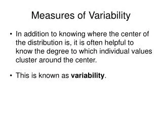
Measures of Central Tendency and Variability So far, we have used very basic characterizations of distributions • Number of modes (unimodal, bimodal, multimodal) • Skew (positive or negative) & Symmetry We need a way to characterize these same distributions quantitatively (using numbers). This allows us to compare distributions. We can describe distributions using two categories of measures: • Measures of Central Tendency • mean, median, mode • Measures of Variability • range, standard deviation, variance
Measures of Central Tendency(where all the action is) Mean-The average of all the scores. The sum of all the scores divided by the number of scores. Example: x : {1, 3, 4, 8 } Σ x (1 + 3 + 4 + 8)16 N 4 4 = = = 4 m The mean is denoted differently depending on the type of data from which it comes: Population mean = μ (pronounced “myou”) __ Sample mean = x (spoken as “x-bar”)
The median is the “middle score” Median – The score that falls in the exact middle of the distribution. (Half the scores are lower and half higher than the median. x = {5, 6, 2, 3, 1, 9, 8, 0, 2, 4, 5} First, arrange the numbers in ascending order: x = {0, 1, 2, 2, 3, 4, 5, 5, 6, 8, 9} Find the number that falls in the middle. For an even number of scores, average the two middle numbers. x = {0, 1, 1, 2, 2, 3, 4, 5, 5, 6, 8, 9}
Mode – The score that occurs most frequently. The score with the highest FREQUENCY. Example: 1, 3, 1, 5, 2, 1, 1, 8, 2, 3, 1, 1, 1, 0, 1, 3, 2, 1, 1, 1
Mode – The score that occurs most frequently. The score with the highest FREQUENCY. Example: 1, 3, 1, 5, 2, 1, 1, 8, 2, 3, 1, 1, 1, 0, 1, 3, 2, 1, 1, 1
Relations between measures of central tendency describe score distribution shape : Skewness When the mean, median, and mode agree, you have symmetry. Pos Skew: Mean > Median Pos Skew: Mean < Median
x 1 0 3 Review of Summation: x: {1, 0, 3} y: {2, 5, 1} x y 1 2 0 5 3 1 Sx = 1 + 0 + 3 = 4 Sx2 = 1 + 0 + 9 = 10 (Sx)2 = (1 + 0 + 3)2 = 42 = 16 S 3x = 3(1) + (3)0 + (3)3 = 3 + 0 + 9 = 12 S xy = 1(2) + (0)5 + (3)1 = 2 + 0 + 3 = 5 (Sx)(Sy) = (1+0+3)(2+5+1) = (4)(8) = 32
Measures of variability: (how clustered or spread out the distribution is) Range - The maximum difference in the data (Max-Min score) Standard Deviation -The average amount that the scores deviate from the mean. Variance - Similar to the standard deviation but with special properties.
The Range Contestant # Canoli Eaten 1 4 2 5 3 6 4 6 5 7 6 8 7 8 8 9 9 10 10 10 11 10 12 10 13 11 14 11 15 11 16 12 17 12 18 14 19 14 20 14 21 16 22 16 23 21 Minimum = 4 Maximum = 21 Range = Maximum - Minimum = 21 - 4 = 17
Standard Deviation: example How much does each score in the sample differ from the average score? The amount by which each score differs from the mean is called its deviation.
Standard Deviation (population) Raw vs. Deviation Scores How do you suppose we would go about finding the AVERAGE amount by which each score DEVIATES from the mean? x: { 1, 2, 3, 2} x 1 2 3 2 μ 2 2 2 2 x – μ -1 0 1 0 (x – μ)2 1 0 1 0 Σ(x-μ)2 ]- Sum of squares (SS) √ Σ(x-μ)2 _______ N SS N 2 4 = = √ √ = .7071 = .71 “deviation method” s = .71
Standard Deviation (sample) x: { 1, 2, 3, 2} _ _ _ _ x 2 2 2 2 x – x -1 0 1 0 x 1 2 3 2 (x – x)2 1 0 1 0 Σ(x-x)2 ]- Sum of squares (SS) _ √ Σ(x-x)2 _______ N-1 SS N-1 2 3 = = √ √ = .8165 = .82 “deviation method” s = .82
The “raw scores method” is an easier way to calculate the Sum of Squares (SS) Remember, s = s = SS N-1 SS N “raw scores method” (Sx)2 √ √ __ __ SS = Sx2 N
Finding the standard deviation using the “raw scores method” for finding the Sum of Squares (SS) _________ x 1 2 3 2 x2 1 4 9 4 SS = 2 (Sx)2 (8)2 Sx = Sx2 = 8 __ __ __ __ SS = 18 SS = Sx2 18 N 4
Remember: Finding the standard deviation using the “raw scores method” for finding the Sum of Squares (SS) _________ POPULATION: SAMPLE: x 1 2 3 2 x2 1 4 9 4 SS = 2 (Sx)2 (8)2 √ √ Sx = Sx2 = 8 __ __ __ __ SS = Sx2 SS = 18 18 4 N s = s = 2 4 2 3 s = .82 s = .71
Summary Slide for Standard Deviation POPULATION: SAMPLE:
Revisiting Pizza… s = 1.16 s = .88
Kurtosis Are all unimodal, symmetrical distributions normal? NO.
The Normal Distribution and Z-scores • What did you get on your SATs? • Prior to 2005, the highest possible score was 1600 • In 2005, an additional section was added to the SAT, • making the highest possible score a 2400 If my score (I took the SATs in 2002) was a 1400, and my friend’s score (2006) was an 1800, did my friend do better than I did or not? We need to find a way to compare scores from different distributions. We cannot compare the raw scores directly.
600 800 1000 1200 1400 If we know that the particular variable on which our score was measured is NORMALLY distributed: • we can specify HOW MANY standard deviations our score is above or below the mean. • For example: We read on Princeton Review’s website that SAT scores are normally distributed. Using the old scale of measurement, the population mean SAT score was 1000, with a standard deviation of 150 points. m = 1000 s = 150 How many standard deviations away from the mean is a score of 1300? . . . . .
x - m s x - x s 600 800 1000 1200 1400 What about a score of 1325? How many standard deviations is it from the mean? 1325 – 1000 150 1325 = 325 150 = 2.166 = 2.17 The Z-score Measures how extreme or unusual a score is within a population *in units of standard deviation. (this means it tells us exactly HOW MANY standard deviations a score is from the mean). z = for population z = for sample
The Z-score Example: MY SAT score (1400) Population of SAT scores (old grading system): m 1000 pts s 150 pts 1400 – 1000 400 z = 150 150 z = 2.6666 = 2.67 standard deviations above the mean MY friend’s SAT score (1800) Population of SAT scores (new grading system): m 1500 pts s 200 pts 1800 – 1500 300 z = 200 200 z = 1.5000 = 1.50 standard deviations above the mean = =