Download
1 / 20
200 likes | 286 Views
KICKOFF OF ASF DISCUSSIONS. So: @ 1000 km --- 1.3 sec to 6 sec 400 to 1800 meters on a pseudorange @ 1310 km --- up to 8 sec. Official government ASF information is available from: http://chartmaker.ncd.noaa.gov/mcd/loranc.htm BUT …… Only for

E N D
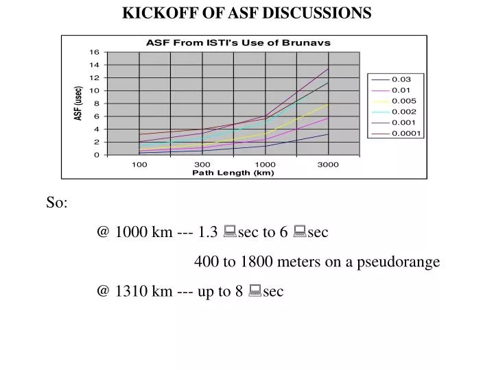
KICKOFF OF ASF DISCUSSIONS So: @ 1000 km --- 1.3 sec to 6 sec 400 to 1800 meters on a pseudorange @ 1310 km --- up to 8 sec
Official government ASF information is available from: http://chartmaker.ncd.noaa.gov/mcd/loranc.htm BUT …… Only for 5930 – X, Y, Z (These are TD ASFs) 7980 – W, X, Y, Z 8970 – X, Y [Note: no W (Malone), no Z (Boise City)] 9940 – W, X, Y 9960 – W, X, Y, Z Note: No CWC, No Alaska, No mid-continent update, not even all of Chain 8970 Moreover, the locations for which these are available are limited
Here’s where you can get some info for 8970-X Note, if a rectangle does not contain at least some CCZ waters, it does not have a table
The charts specifically exclude any sub-sector that does not include CCZ water Note Plumbrook is at 41-22N and 82-39W
Here’s what you get if you transform to position estimates the 8970-X and 8970-Y system sample (a full daytime hour) TDs recorded at Plumbrook over all of 1999 and 2000 --- using no ASFs (aka the model ASF = 0). This site is very close to the CCZ, though on land. However, the USCG Signal Spec claims Loran-C provides 0.25 nmi, 2 drms predictable accuracy throughout CONUS. Careful CG!
Here’s how the same system sample hourly averages throughout 1999 and 2000 plot out as positions with the “nearest” NOAA ASFs applied It seems apparent the “calibration” was done in the summer – which makes sense because of all the shoreside reference system setup work (believed to be maxiran) The failure to get the calibration point in the ellipse may be due to extrapolation, but may also be due to maxiran Note: there are more error components than those shown
For those who don’t recall how we knew the summer values plotted to the SW: Also: when the TD’s increase, you move towards the master (Dana) Here’s what we’d get if we aimed at the MMSE estimate: Though we’re within limits, we have other terms to add. We can and should do better.
This seems to be a better approach – it directly addresses the requirement: minimize the maximum error It thus seems reasonable to suggest the goal should be to measure both the summer and winter extremes – where there is a non-trivial seasonal component. This needs to be predicted with the tool being developed by PIG It should also be clear we need a method to help us estimate the seasonal extremes from measurements taken on our schedule
In this regard, here are some plots from an analysis prompted by discussions with ISTI in the Spring of 2001 The above is with no ASF. Here are corrections from NOAA: The points above 0.25 nmi do not come from the “primary triad” at the associated site. At the same time, this is only the spatial bias. The CG probably misses 0.25 nmi 95% but comes “close enough.” Be careful about 2drms claims with large biases.
ISTI has an algorithm which uses an ASF calculation model suggested by Brunavs. When the results were applied to all the HMS data, the plot on the lest was found. The straight lines are of the form ASF error = k x ASF prediction. Where k = 0.15 and 0.30. The bottom line contains about 56% of the points, the upper line contains about 91% of the points. The graph on the right shows similar results when we omit some Canadian and northern N.E. areas where the conductivity profiles are sparse. The slopes are closer to 11% and 22%. Before mid-March 2002, we thought the goal was 0.3 nmi, 95% CTE and the above results suggested we might get by with some simple prediction algorithms, a mild validation program, and perhaps some concentrated effort where the profiles are sparse.
All the preceding suggests that when we switched to trying for 0.3 nmi at the 99.99999% level, and 0.165 nmi, 95%, a calibration was needed. We can still use the error model (e.g., in the form of ASF error = 0.3 x ASF prediction). However, at least at the calibration points, it seems excessive
Many questions have to be addressed Here are some questions, in the form of answers, for the transmitted signals: 1. The “grid difference” between SAM control and ToT control is significant enough in many places that there will be many places where we could make the requirements, but not if we calibrate under the wrong control method. (T or F?) 2. ToT control is better than SAM control – in a “global sense” (relative to a maximum allowable error) than SAM control – but not by as much what is lost in item 1. (T or F?) 3. Thus, the preference would probably be: (a) calibrate and operate under ToT, (b) calibrate and operate under SAM, (c) calibrate under SAM, operate under ToT – in that order due to increasing error budgets. (Academic exercise, but T or F?) 4. 0.3 nmi/99.99999% and 0.165 nmi/95% are significant enough challenges that it is really important to not have to ponder the above choices – we want to count on ToT all the way. (T or F?)
You can’t always get what you want (but if you try real hard, you just might find you get what you need) – M. Jagger 5. The CG is not equipped to switch to SAM control for many years (T or F?) 6. However, it is possible to do the calibration under “ToT-like” conditions as long as high fidelity ToT measurements can be made, even if they aren’t yet “clutched in.” (T or F?) 7. It may be possible for the CG to make the ToT measurements long before the control method is switched, even before the final equipment suite is installed. If this can be done by the CG, with only a small rise in the error budget, calibration measurements can be adjusted and little is lost (T or F?)
The questions extend to the received signals: 1. We can find the summer and winter extremes at a calibration site if we install a monitor at each such site and leave it for a year or two. (T or F?) 2. It is not practical to install monitors at all calibration data sites where seasonal variations are a concern. (T or F?) 3. The CG has a large network of installed monitor receivers and these have produced data records over many years. (T or F?) 4. Past Loran-C Signal Stability studies efforts have indicated ways which observations obtained over nearby paths can be used to predict seasonal variations with a reasonable (measurable) degree of confidence at nearby sites. (T or F?) 5. All the above suggests a method whereby the variations at nearby fixed monitors is used to predict how far the calibration measurement, at any given time, is from the extreme, and with what confidence.
A break from the questions, for some data indications The 8970-X and 8970-Y system samples have a corr. Coeff. Of 0.978 Can we use this and other paths to predict difference of measurement to extreme? Looks decent but regression analysis shows sigma = 120 nsec and max residual (254 points) = 340 nsec If we are seeing max for 250 points at 3 sigma,this is nearly gaussian. We can reduce this with more “reference sites” but how many can we count on?
Let’s remember this is an analysis of a set of “very busy” sums: x = X + prediction error on Dana-to-Plumbrook path - prediction error on Dana-to-Dunbar path + prediction error on Seneca-to-Dunbar path - prediction error on Seneca-to-Plumbrook path vs y = Y + prediction error on Dana-to-Plumbrook path - prediction error on Dana-to-Dunbar path + prediction error on Baudette-to-Dunbar path - prediction error on Baudette-to-Plumbrook path For 5.33 sigma = 640 nsec, we might cut this in half in reading just TOAs. Can we cut the resulting 320 nsec down more?
Consider Plumbrook. What would we be trying to estimate? Winter: Estimate (Extreme – Day X reading)Cal Site from places where Extremes and Day X readings are known Predict for: (A) Path from Dana to Ohio Site N (B) Path from Seneca to Site N (C) Path from Baudette to Path N Use: (1) Dana-Seneca Baseline* (2) Dana-to-Dunbar & Seneca-to-Dunbar Paths* (3) Dana-Baudette Baseline** (4) Dana-to-Dunbar & Seneca-to-Dunbar Paths** (5) Dana-to-Plumbrook & Seneca-to-Plumbrook Paths*** (6) Dana-to-Plumbrook & Baudette-to-Plumbrook Paths*** ‘*BL End differences/2‘*BL Averages/2‘*Using ED variations
Regrettably, that’s only 6 paths If we could get LRS’s in and get the data, we could also have: (7) Dana-to-Carolina Beach Path (8) Dana-to-Nantucket Path (9) Dana-to-Caribou Path (10) Seneca-to-Baudette Path If we could get more readings from the Lormonsites: (11) Dana-to-Plumbrook & Nantucket-to-Plumbrook (12) Dana-to-Plumbrook & Carolina Beach-to-Plumbrook Maybe some others. Perhaps even with no other a priori information, this might give us almost a factor of 3.5 mitigation Should we try to look at weather?
Summary: The calibration needs to take into account the seasonal variations For paths west of the Rockies and in the SEUS, such variations are small In the Great Lakes and NEUS areas, we need special care It is impossible to monitor always everywhere The best approach seems to be to estimate the summer and winter extremes by at least summer and winter measurement and to statistically project those measurements using a combination of weather data and CG fixed site receiver measurements in the region The methodology needs to be developed


![Pass Your ASF Exam with Authentic ASF Dumps [PDF]](https://cdn4.slideserve.com/7887664/slide1-dt.jpg)