Download

1 / 21
210 likes | 337 Views
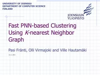
Fast PNN-based Clustering Using K -nearest Neighbor Graph. Pasi Fränti, Olli Virmajoki and Ville Hautamäki 15.11.2003. UNIVERSITY OF JOENSUU DEPARTMENT OF COMPUTER SCIENCE FINLAND. Agglomerative clustering. N = 22 ( data vectors ) M = 3 ( final clusters ). PNN method for clustering.

E N D
Fast PNN-based Clustering Using K-nearest Neighbor Graph Pasi Fränti, Olli Virmajoki and Ville Hautamäki 15.11.2003 UNIVERSITY OF JOENSUU DEPARTMENT OF COMPUTER SCIENCE FINLAND
Agglomerative clustering N = 22 ( data vectors ) M = 3 ( final clusters )
PNN method for clustering Merge cost: Local optimization strategy:
NN search O(N) searches with the PNN method O(k) searches with the graph structure ( k=3 )
Graph-based PNN • Based on the exact PNN • Search is limited only to the clusters that are connected by the graph structure • Reduces the time complexity of every search from O(N) to O(k) (Example: N=4096, k=3-5)
Structure of the Graph-PNN GraphPNN(X, M)S FOR i 1 to N DO si {xi}; FOR DO Find k nearest neighbors; REPEAT (sa, sb) GetNearestClustersInGraph(S); sab Merge(sa, sb); Search the k nearest neighbors for sab; Update the nodes that had sa and sb as neighbors; UNTIL |S|=M;
Sample graph (k=3 and k=4) (k=3) (k=4) Isolated component
(k=3) Steps Distance calculations Fast PNN 81 960 610 40 166 328 Graph-PNN simple 50 468 663 47 370 Graph-PNN double linked 517 905 47 413 Observed number of steps and distance calculations for Bridge
Creation of nearest neighbor graph • Brute force O(N 2) • MPS ! • Divide-and-conquer (to be considered)
Bridge (256256) d = 16 N = 4096 M = 256 Miss America (360288) d = 16 N = 6480 M = 256 House (256256) d = 3 N = 34112 M =256 Image datasets
BIRCH datasets Datasets BIRCH1, BIRCH2 and BIRCH3 d = 2 N = 100 000 M = 100
Two-dimensional datasets Datasets S1, S2, S3 and S4 d = 2 N = 5 000 M = 15
Birch datasets BIRCH 1 BIRCH 2 BIRCH 3 Time MSE Time MSE Time MSE Fast PNN Full search > 4 h 4.73 > 4 h 2.28 > 4 h 1.96 +PDS+MPS+Lazy 2397 4.73 2115 2.28 2316 1.96 Graph-PNN + GLA Limited search MPS 41 4.64 16 2.28 44 1.90 Comparison of the Graph-PNN (k=5) with other methods
Conclusions • Small neighborhood size (k=3-5) can produce clustering with similar quality to that of full search. • The number of steps and distance calculations is remarkable lower than that of the exact PNN. • Graph creation is the bottleneck of the algorithm.