Download
1 / 39
390 likes | 506 Views
Loop Analysis (7.8) Circuits with Op-Amps (3.3). Dr. Holbert October 9, 2001. Another Analysis Example. We will re-analyze the possible implementation of an AM Radio IF amplifier. We will solve for output voltages using mesh analysis this time.

E N D
Loop Analysis (7.8)Circuits with Op-Amps (3.3) Dr. Holbert October 9, 2001 ECE201 Lect-13
Another Analysis Example • We will re-analyze the possible implementation of an AM Radio IF amplifier. • We will solve for output voltages using mesh analysis this time. • This circuit is a bandpass filter with center frequency 455kHz and bandwidth 40kHz. ECE201 Lect-13
IF Amplifier 100pF 4kW 100pF 80kW – + + – + – 1V 0 Vx 100Vx Vout 160W + – ECE201 Lect-13
Mesh AC Analysis • Use AC steady-state analysis. • Use a frequency of w=2p 100,000. ECE201 Lect-13
-j15.9kW 4kW -j15.9kW 80kW – + + – + – 1V 0 Vx 100Vx Vout 160W + – Impedances ECE201 Lect-13
-j15.9kW I3 4kW -j15.9kW 80kW – + + – + – 1V 0 Vx 100Vx Vout 160W I1 I2 + – Mesh Analysis ECE201 Lect-13
KVL Around Loop 1 ECE201 Lect-13
KVL Around Loop 2 ECE201 Lect-13
KVL Around Loop 2 (Cont) ECE201 Lect-13
KVL Around Loop 3 ECE201 Lect-13
Solve Equations I1 = 239.9 + j0.23 mA I2 = -12.36 + j5.98 mA I3 = -12.54 + j3.46 mA ECE201 Lect-13
Solve for Vout ECE201 Lect-13
|Vout| as a function of w ECE201 Lect-13
Class Example • Learning Extension E7.14(a) ECE201 Lect-13
Op Amps • Op Amp is short for operational amplifier. • An operational amplifier is modeled as a voltage controlled voltage source. • An operational amplifier has a very high input impedance and a very high gain. ECE201 Lect-13
Use of Op Amps • Op amps can be configured in many different ways using resistors and other components. • Most configurations use feedback. ECE201 Lect-13
Applications of Op Amps • Amplifiers provide gains in voltage or current. • Op amps can convert current to voltage. • Op amps can provide a buffer between two circuits. • Op amps can be used to implement integrators and differentiators. • Lowpass and bandpass filters. ECE201 Lect-13
+ - The Op Amp Symbol High Supply Non-inverting input Output Inverting input Ground Low Supply ECE201 Lect-13
The Op Amp Model v+ Non-inverting input + vo Rin + – Inverting input – A(v+ -v- ) v- ECE201 Lect-13
Typical Op Amp • The input resistance Rin is very large (practically infinite). • The voltage gain A is very large (practically infinite). ECE201 Lect-13
“Ideal” Op Amp • The input resistance is infinite. • The gain is infinite. • The op amp is in a negative feedback configuration. ECE201 Lect-13
The Basic Inverting Amplifier R2 R1 – + – + + Vin Vout – ECE201 Lect-13
Consequences of the Ideal • Infinite input resistance means the current into the inverting input is zero: i- = 0 • Infinite gain means the difference between v+ and v- is zero: v+ - v- = 0 ECE201 Lect-13
Solving the Amplifier Circuit Apply KCL at the inverting input: i1 + i2 + i-=0 R2 i2 R1 – i1 i- ECE201 Lect-13
KCL ECE201 Lect-13
Solve for vout Amplifier gain: ECE201 Lect-13
Recap • The ideal op-amp model leads to the following conditions: i- = 0 = i+ v+ = v- • These conditions are used, along with KCL and other analysis techniques, to solve for the output voltage in terms of the input(s). ECE201 Lect-13
Where is the Feedback? R2 R1 – + – + + Vin Vout – ECE201 Lect-13
Review • To solve an op-amp circuit, we usually apply KCL at one or both of the inputs. • We then invoke the consequences of the ideal model. • The op amp will provide whatever output voltage is necessary to make both input voltages equal. • We solve for the op-amp output voltage. ECE201 Lect-13
The Non-Inverting Amplifier + + – + – vin vout R2 R1 – ECE201 Lect-13
KCL at the Inverting Input + + – + – i- vin vout i1 i2 R2 R1 – ECE201 Lect-13
KCL ECE201 Lect-13
Solve for Vout ECE201 Lect-13
A Mixer Circuit R1 Rf + – R2 v1 – + – + + v2 vout – ECE201 Lect-13
KCL at the Inverting Input R1 Rf i1 if + – R2 v1 i2 – i- + – + + v2 vout – ECE201 Lect-13
KCL ECE201 Lect-13
KCL ECE201 Lect-13
Solve for Vout ECE201 Lect-13
Class Example • Learning Extension E3.16 ECE201 Lect-13