Download
1 / 42
420 likes | 472 Views
CSC 213 – Large Scale Programming. Lecture 24: Merge Sort –or– Lessons from Roman Empire. Today’s Goals. Review past discussion of data sorting algorithms Weaknesses of past approaches & when we use them Can we find limit to how long sorting needs?

E N D
CSC 213 – Large Scale Programming Lecture 24:Merge Sort –or–Lessons from Roman Empire
Today’s Goals • Review past discussion of data sorting algorithms • Weaknesses of past approaches & when we use them • Can we find limit to how long sorting needs? • What does this mean for sorting & those past sorts • Get good idea of how merge sort is executed • What is algorithm and what will this require? • What are execution trees & how they show runtime?
Ghosts of Sorts Past • We have already seen & discussed 4 sorts • Bubble-sort-- O(n2) time sort; slowest sort • Selection-sort-- O(n2) time sort; PQ concept • Insertion-sort-- O(n2) time sort; PQ concept • Heap-sort-- O(n log n) time sort; requires PQ • All of these sorts of limited usefulness
Ghosts of Sorts Past • We have already seen & discussed 4 sorts • Bubble-sort-- O(n2) time sort; slowest sort • Selection-sort-- O(n2) time sort; PQ concept • Insertion-sort-- O(n2) time sort; PQ concept • Heap-sort-- O(n log n) time sort; requires PQ • All of these sorts of limited usefulness
Counting Comparisons • Consider sort as a path in a decision tree • Nodes are single decision needed for sorting Is xi > xj ? yes no
Counting Comparisons • Consider sort as a path in a decision tree • Nodes are single decision needed for sorting • Traveling from root to leaf sorts data • Tree’s height is lower-bound on sorting complexity
Decision Tree Height • Unique leaf for each ordering of data initially • Needed to ensure we sort different inputs differently • Consider 4, 5as data to be sorted using a tree • Could be entered in 2 possible orders: 4, 5or5, 4 • Need two leaves for this sort unless (4 < 5) == (5 < 4)
Decision Tree Height • Unique leaf for each ordering of data initially • Needed to ensure we sort different inputs differently • Consider 4, 5as data to be sorted using a tree • Could be entered in 2 possible orders: 4, 5or5, 4 • Need two leaves for this sort unless (4 < 5) == (5 < 4) • For sequence of n numbers, can arrange n! ways • Tree with n! leaves needed to sort n numbers • Given this many leaves, what is height of the tree?
Decision Tree Height • With n! external nodes, binary tree’s height is:
The Lower Bound • But what does O(log(n!))equal?n! = n * n-1 * n -2 * n-3 * n/2 * … * 2 * 1n!≤(½*n)½*n(½of series is larger than ½*n) log(n!)≤log((½*n)½*n) log(n!)≤½*n* log(½*n) O(log(n!)) ≤O(½*n * log(½*n))
The Lower Bound • But what does O(log(n!))equal?n! = n * n-1 * n -2 * n-3 * n/2 * … * 2 * 1n!≤(½*n)½*n(½of series is larger than ½*n) log(n!)≤log((½*n)½*n) log(n!)≤½*n* log(½*n) O(log(n!)) ≤O(½*n * log(½*n))
The Lower Bound • But what does O(log(n!))equal?n! = n * n-1 * n -2 * n-3 * n/2 * … * 2 * 1n!≤(½*n)½*n(½of series is larger than ½*n) log(n!)≤log((½*n)½*n) log(n!)≤½*n* log(½*n) O(log(n!)) ≤O(n log n)
Lower Bound on Sorting • Smallest number of comparisonsis tree’s height • Decision tree sorting n elements has n! leaves • At least log(n!) height needed for this many leaves • As we saw, this simplifies to at most O(n log n) height • O(n log n) time needed to compare data! • Means that heap-sort is fastest possible (in big-Oh) • Pain-in-the- to code & requires external heap
Lower Bound on Sorting • Smallest number of comparisonsis tree’s height • Decision tree sorting n elements has n! leaves • At least log(n!) height needed for this many leaves • As we saw, this simplifies to at most O(n log n) height • O(n log n) time needed to compare data! • Means that heap-sort is fastest possible (in big-Oh) • Pain-in-the- to code & requires external heap • Is there a simple sort using only Sequence?
Julius, Seize Her! • Formula to Roman success • Divide peoples before an attack • Then conquer weakened armies • Common programming paradigm • Divide: split into 2 partitions • Recur:solve for partitions • Conquer:combine solutions
Divide-and-Conquer • Like all recursive algorithms, need base case • Has immediate solution to a simple problem • Work is not easy and sorting 2+ items takes work • Already sorted 1 item since it cannot be out of order • Sorting a list with 0 items even easer • Recursive step simplifies problem & combines it • Begins by splitting data into two equal Sequences • Merges subSequencesafter they have been sorted
Merge-Sort AlgorithmmergeSort(Sequence<E> S, Comparator<E>C) ifS.size() <2then // Base case return S else // Recursive case //Split Sinto two equal-sized partitionsS1andS2 mergeSort(S1,C) mergeSort(S2,C) S merge(S1,S2,C) returnS
Merging Sorted Sequences Algorithmmerge(S1,S2,C)Sequence<E> retVal= //Code instantiating a Sequencewhile!S1.isEmpty() && ! S2.isEmpty()ifC.compare(S1.get(0),S2.get(0)) < 0retVal.insertLast(S1.removeFirst())elseretVal.insertLast(S2.removeFirst())endifendwhile!S1.isEmpty()retVal.insertLast(S1.removeFirst())endwhile!S2.isEmpty() retVal.insertLast(S2.removeFirst()) endreturn retVal
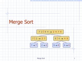
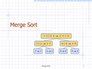
Execution Tree • Depicts divide-and-conquer execution • Recursive call represented by each oval node • Original Sequence shown at start • At the end of the oval, sorted Sequence shown • Initial call at root of the (binary) tree • Bottom of the tree has leaves for base cases
Execution Example • Not in a base case 7 2 9 4 3 8 6 1 1 2 3 4 6 7 8 9
Execution Example • Not in a base case, so split into S1 & S2 7 2 9 4 3 8 6 1 1 2 3 4 6 7 8 9
Execution Example • Not in a base case, so split into S1 & S2 7 2 9 4 3 8 6 1 1 2 3 4 6 7 8 9
Execution Example • Recursively call merge-sort on S1 7 2 9 4 3 8 6 1 1 2 3 4 6 7 8 9
Execution Example • Recursively call merge-sort on S1 7 2 9 4 3 8 6 1 1 2 3 4 6 7 8 9 7 2 9 4 2 4 7 9
Execution Example • Not in a base case, so split into S1 & S2 7 2 9 4 3 8 6 1 1 2 3 4 6 7 8 9 7 2 9 4 2 4 7 9
Execution Example • Not in a base case, so split into S1 & S2 7 2 9 4 3 8 6 1 1 2 3 4 6 7 8 9 7 2 9 4 2 4 7 9
Execution Example • Recursively call merge-sort on S1 7 2 9 4 3 8 6 1 1 2 3 4 6 7 8 9 7 2 9 4 2 4 7 9
Execution Example • Recursively call merge-sort on S1 7 2 9 4 3 8 6 1 1 2 3 4 6 7 8 9 7 2 9 4 2 4 7 9 7 2 2 7
Execution Example • Still no base case, so split again & recurse on S1 7 2 9 4 3 8 6 1 1 2 3 4 6 7 8 9 7 2 9 4 2 4 7 9 72 2 7 7 7
Execution Example • Enjoy the base case – literally no work to do! 7 2 9 4 3 8 6 1 1 2 3 4 6 7 8 9 7 2 9 4 2 4 7 9 72 2 7 77
Execution Example • Recurse on S2and solve for this base case 7 2 9 4 3 8 6 1 1 2 3 4 6 7 8 9 7 2 9 4 2 4 7 9 72 2 7 77 22
Execution Example • Merge the two solutions to complete this call 7 2 9 4 3 8 6 1 1 2 3 4 6 7 8 9 7 2 9 4 2 4 7 9 72 2 7 77 22
Execution Example • Recurse on S2and sort this subSequence 7 2 9 4 3 8 6 1 1 2 3 4 6 7 8 9 7 2 9 4 2 4 7 9 72 2 7 9 4 4 9 77 22
Execution Example • Split into S1 & S2and solve the base cases 7 2 9 4 3 8 6 1 1 2 3 4 6 7 8 9 7 2 9 4 2 4 7 9 72 2 7 94 4 9 77 22 9 9 44
Execution Example • Merge the 2 solutions to sort this Sequence 7 2 9 4 3 8 6 1 1 2 3 4 6 7 8 9 7 2 9 4 2 4 7 9 72 2 7 944 9 77 22 9 9 44
Execution Example • I feel an urge, an urge to merge 7 2 9 4 3 8 6 1 1 2 3 4 6 7 8 9 7 2 9 4 2 4 7 9 72 2 7 944 9 77 22 9 9 44
Execution Example • Let's do the merge sort again! (with S2) 7 2 9 4 3 8 6 1 1 2 3 4 6 7 8 9 7 2 9 4 2 4 7 9 3 8 6 11 3 6 8 72 2 7 944 9 77 22 9 9 44
Execution Example • Let's do the merge sort again! (with S2) 7 2 9 4 3 8 6 1 1 2 3 4 6 7 8 9 7 2 9 4 2 4 7 9 3 8 6 11 3 6 8 72 2 7 944 9 38 3 8 77 22 9 9 44 33 88
Execution Example • Let's do the merge sort again! (with S2) 7 2 9 4 3 8 6 1 1 2 3 4 6 7 8 9 7 2 9 4 2 4 7 9 3 8 6 11 3 6 8 72 2 7 944 9 38 3 8 611 6 77 22 9 9 44 33 88 66 11
Execution Example • Let's do the merge sort again! (with S2) 7 2 9 4 3 8 6 1 1 2 3 4 6 7 8 9 7 2 9 4 2 4 7 9 3 8 6 11 3 6 8 72 2 7 944 9 38 3 8 611 6 77 22 9 9 44 33 88 66 11
Execution Example • Merge the last call to get the final result 7 2 9 4 3 8 6 1 1 2 3 4 6 7 8 9 7 2 9 4 2 4 7 9 3 8 6 11 3 6 8 72 2 7 944 9 38 3 8 611 6 77 22 9 9 44 33 88 66 11
For Next Lecture • New weekly assignment for week was posted • Discussing sorts which have few concepts to code • Will return soon enough; do not worry about it • Keep reviewing requirements for program #2 • Preliminary deadlines arrive before final version • Time spent on requirements & design saves coding • Reading on quick sort for this Friday • Guess what? It can be really, really, quick • Severe drawbacks also exist; read to understand this