Download
1 / 61
630 likes | 743 Views
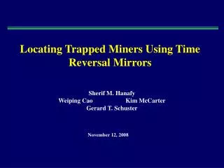
Hydro-frac Source Estimation by Time Reversal Mirrors. Weiping Cao and C. Boonyasiriwat. UTAM, The University of Utah. Outline. Motivation. Methodology. Numerical Examples. Conclusions. Outline. Motivation. Methodology. Numerical Examples. Conclusions. Motivation.

E N D
Hydro-frac Source Estimation by Time Reversal Mirrors Weiping Cao and C. Boonyasiriwat UTAM, The University of Utah
Outline • Motivation • Methodology • Numerical Examples • Conclusions
Outline • Motivation • Methodology • Numerical Examples • Conclusions
Motivation • Hydro-frac is important for oil recovery operations; • Using time reversal mirror (TRM) method, only a local velocity model near the well needed; • Potential for super-resolution and super-stacking properties from TRM.
Outline • Motivations • Methodology • Numerical Examples • Conclusions
Methodology • TRM imaging; • Apply TRM imaging to locating hydro-fracs by wavefield extrapolation; • Detailed implementation.
Multiples Primary TRM Imaging Time Reversal Mirror Time Image source location with natural Green’s functions No velocity model needed
TRM imaging g : passive data generated by hydro-fracs Problem: finding Apply TRM to Locating Hydro-fracs s Solution: extrapolate VSP or seismic while drilling (SWD) data.
Forward extrapolation: Backward extrapolation: : convolution g x : crosscorrelation go Extrapolate VSP or SWD Data to obtain g go x Only a local vel. model needed
Methodology Summary for the implementation: Record VSP or SWD data as natural GF; Extrapolate VSP or SWD data to obtain semi-natural GFs between surface and image points using the local velocity model near the well; Cross-correlate these semi-natural GFs to the passive seismic data generated by hydro-fracs.
Outline • Motivation • Methodology Numerical Examples • Conclusions
Numerical Examples Synthetic Tests with SEG/EAGE Salt Model: Hydro-frac imaging with correct source excitation times; Hydro-frac imaging with strong background noise; Hydro-frac imaging with incorrect source excitation times;
SEG/EAGE Salt Model 0 4 (km/s) Z (km) 2 (km/s) 3.5 0 16 X (km) Synthetic Data Generation Synthetic data: RVSP or SWD data, Passive seismic gathers
Image with Correct Source Excitation Times TRM imaging with forward extrapolation Actual hydro-frac location: (10 km, 3.4 km) 3.2 3.5 km/s Z (km) 3.7 2.5 8 12 X (km)
Image with Correct Source Excitation Times TRM imaging with backward extrapolation Actual hydro-frac location: (10 km, 3.01 km) 2.7 3.1 km/s Z (km) 3.2 2.3 8 12 X (km)
Image with Strong Background Noise Synthetic Passive Gather Noisy Gather: S/N =10,495 0 0 Time (s) Time (s) 6 6 0 Receiver X (km) 15 0 Receiver X (km) 15 Actual hydro-frac source location: (10 km, 3.01 km)
Image with Strong Background Noise TRM Image from the Noisy Gather 2.7 1 Z (km) -0.5 3.2 8 12 X (km)
Image with Strong Background Noise TRM Image from the Noisy Gather: S / N =1 / 10496 2.7 1 Z (km) -0.5 3.2 8 12 X (km)
3.2 20 ms advance Z (km) 3.7 12 8 X (km) 3.2 Exact source excitation time Z (km) 3.7 12 8 X (km) 3.2 20 ms delay Z (km) 3.7 12 8 X (km) Image with Incorrect Source Excitation Times
Outline • Motivation • Methodology • Numerical Examples Conclusions
Conclusions TRM is applied to locate hydro-fracs with VSP or SWD data, and provide accurate images when we use exact source excitation times. TRM images show strong resilience to white noise. TRM images are sensitive to source excitation times. 2-D median assumption.
Acknowledgments We thank the 2007 UTAM sponsors for the support.
Image with Strong Background Noise 1 2.7 Z (km) -0.5 3.2 8 12 X (km)
Image with Strong Background Noise 1 2.7 Z (km) -0.5 3.2 8 12 X (km)
Image with Correct Source Excitation Times 3.2 3.5 km/s Z (km) 3.7 2.5 8 12 X (km)
Interferometric Imaging Implementation Step 1: Extrapolate of VSP data Step2: Image hydro-fracture sources
Outline • Motivations • Methodology • Numerical Examples • Conclusions
Numerical Examples SEG/EAGE Salt Model 0 Z (km) 3.5 0 16 X (km)
Multiples Primary TRM Imaging Time Reversal Mirror Time Image source location with natural Green’s functions No velocity model needed
Multiples Primary TRM Imaging Time Reversal Mirror Time Image source location with natural Green’s functions No velocity model needed
: passive data generated by hydro-fracs Apply TRM to Locating Hydro-fracs Hydro-frac Location Problem: finding Solution: extrapolate VSP or seismic while drilling (SWD) data.