Download

1 / 55
550 likes | 745 Views
Short Term Scheduling. Characteristics. Planning horizon is short Multiple unique jobs (tasks) with varying processing times and due dates Multiple unique jobs sharing the same set of resources (machines) Time is treated as continuous (not discretized into periods)

E N D
Characteristics • Planning horizon is short • Multiple unique jobs (tasks) with varying processing times and due dates • Multiple unique jobs sharing the same set of resources (machines) • Time is treated as continuous (not discretized into periods) • Varying objective functions
Characteristics (Continued…) • Common in make-to-order environments with high product variety • Common as a support tool for MRP in generating detailed schedules once orders have been released
Example • Two jobs, A and B • Two machines M1 and M2 • Jobs are processed on M1 and then on M2 • Job A: 9 minutes on M1 and 2 minutes on M2 • Job B: 4 minutes on M1 and 9 minutes on M2
Challenge As the number of jobs increases, complete enumeration becomes difficult: 3! = 6, 4! = 24, 5! = 120, 6! = 720, … 10! =3,628,800, while 13! = 6,227,020,800 25!= 15,511,210,043,330,985,984,000,000
Classification of Scheduling Problems • Number of jobs • Number of machines • Type of production facility • Single machine • Flow shop • parallel machines • job shop • Job arrivals • Static • Dynamic • Performance measures
A Single Machine Example Jobs 1 2 3 4 5 6 Processing time, pj 12 8 3 10 4 18 Release time, rj -20 -15 12 -10 3 2 Due date, dj10 2 72 -8 8 60
The Single Machine Problem Single machine scheduling problems seek an optimal sequence (for a given criterion) in which to complete a given collection of jobs on a single machine that can accommodate only one job at a time.
Decision Variables • xj: time job j is started (relative to time 0 = now), xj max(0, rj) for all values of j.
Sequencing constraints - (start time of j)+ (processing time of j) < start time of j’ or - (start time of j’)+ (processing time of j’) < start time of j
Sequencing constraints - (start time of j)+ (processing time of j) start time of j’ or - (start time of j’)+ (processing time of j’) start time of j xj+ pj xj’ or xj’ + pj’ xj
Disjunctive variables - Introduce disjunctive variables yjj’, yjj’ = 1 if job j is scheduled before job j’ and yjj’ = 0 otherwise. xj+ pj xj’ + M(1 - yjj’), xj’+ pj’ xj + Myjj’, for all pairs of j and j’ (for every j and every j’ > j), M is a large positive constant
Due date constraints xj+ pj dj for all values of j
Example Jobs 1 2 3 Processing time 15 6 9 Release time 5 10 0 Due date 20 25 36 Start time 9 24 0
Formulation: Minimizing Makespan (Maximum Completion Time)
A Formulation with a Linear Objective Function
Similar formulations can be constructed with other min-max objective functions, such as minimizing maximum lateness or maximum tardiness. • Other objective functions involving minimizing means (other than mean tardiness) are already linear.
The Job Shop Scheduling Problem • N jobs • M Machines • A job j visits in a specified sequence a subset of the machines
Notation • pjm: processing time of job j on machine m, • xjm:start time of job j on machine m, • yj,j’,m = 1 if job j is scheduled before job j’ on machine m, • M(j): The subset of the machines visited by job j, • SS(m, j): the set of machines that job j visits after visiting machine m
Solution Methods • Small to medium problems can be solved exactly (to optimality) using techniques such as branch and bound and dynamic programming • Structural results and polynomial (fast) algorithms for certain special cases • Large problems in general may not solve within a reasonable amount of time (the problem belongs to a class of combinatorial optimization problems called NP-hard) • Large problems can be solved approximately using heuristic approaches
Single Machine Results • Makespan • Not affected by sequence • Average Flow Time • Minimized by performing jobs according to the “shortest processing time” (SPT) order • Average Lateness • Minimized by performing in “shortest processing time” (SPT) order • Maximum Lateness (or Tardiness) • Minimized by performing in “earliest due date” (EDD) order. • If there exists a sequence with no tardy jobs, EDD will do it
Single Machine Results (Continued…) • Average Weighted Flow Time • Minimized by performing according to the “smallest processing time ratio” (processing time/weight) order • Average Tardiness • No simple sequencing rule will work
Two Machine Results • Given a set of jobs that must go through a sequence of two machines, what sequence will yield the minimum makespan?
Johnson’s Algorithm A Simple algorithm (Johnson 1954): 1. Sort the processing times of the jobs on the two machines in two lists. 2. Find the shortest processing time in either list and remove the corresponding job from both lists. • If the job came from the first list, place it in the first available position in the sequence. • If the job came from the second list, place it in the last available position in sequence. 3. Repeat until are all jobs have been sequenced. The resulting sequence minimizes makespan.
Johnson’s Algorithm Example • Data: • Iteration 1: min time is 4 (job 1 on M1); place this job first and remove from both lists:
Johnson’s Algorithm Example (Continued…) • Iteration 2: min time is 5 (job 3 on M2); place this job last and remove from lists: • Iteration 3: only job left is job 2; place in remaining position (middle). • Final Sequence: 1-2-3 • Makespan: 28
Gantt Chart for Johnson’s Algorithm Example Short task on M2 to “clear out” quickly. Short task on M1 to “load up” quickly.
Three Machine Results • Johnson’s algorithm can be extended to three machines by creating two composite machines (M1* = M1 + M2) and (M2* = M2 + M3) and then applying Johnson’s algorithm to these two machines • Optimality is guaranteed only when certain conditions are met • smallest processing time on M1 is greater or equal than largest processing on machine 2, or • smallest processing time on M3 is greater or equal than largest processing on machine 2
Multi-Machine Results • Generate M-1 pairs of dummy machines • Example: with 4 machines, we have the following three pairs (M1, M4), (M1+M2, M3+M4), (M1+M2+M3, M2+M3+M4) • Apply Johnson’s algorithm to each pair and select the best resulting schedule out of the M-1 schedules generated • Optimality is not guaranteed.
Dispatching Rules • In general, simple sequencing rules (dispatching rules) do not lead to optimal schedules. However, they are often used to solve approximately (heuristically) complex scheduling problems. • Basic Approach • Decompose a multi-machine problem (e.g., a job shop scheduling problem) into sub-problems each involving a single machine. • Use a simple dispatching rule to sequence jobs on each of these machines.
Example Dispatching Rules • FIFO – simplest, seems “fair”. • SPT – Actually works quite well with tight due dates. • EDD – Works well when jobs are mostly the same size. • Critical ratio (time until due date/work remaining) - Works well for tardiness measures • Many (100’s) others.
Heuristics Algorithms • Construction heuristics • Use a procedure (a set of rules) to construct from scratch a good (but not necessarily optimal) schedule • Improvement heuristics • Starting from a feasible schedule (possibly obtained using a construction heuristic), use a procedure to further improve the schedule
Example: A Single Machine with Setups • N jobs to be scheduled on a single machine with a sequence dependent setup preceding the processing of each job. • The objective is to identify a sequence that minimizes makespan. • The problem is an instance of the Traveling Salesman Problem (TSP). • The problem is NP-hard (the number of computational steps required to solve the problem grow exponentially with the number of jobs).
A Heuristic Algorithm • Greedy heuristic: Start with an arbitrary job from the set of N jobs. Schedule jobs subsequently based on “next shortest setup time.”
A Heuristic Algorithm • Greedy heuristic: Start with an arbitrary job from the set of N jobs. Schedule jobs subsequently based on “next shortest setup time.” • Improved greedy heuristic: Evaluate sequences with all possible starting jobs (N different schedules). Choose schedule with the shortest makespan.
A Heuristic Algorithm • Greedy heuristic: Start with an arbitrary job from the set of N jobs. Schedule jobs subsequently based on “next shortest setup time.” • Improved greedy heuristic: Evaluate sequences with all possible starting jobs (N different schedules). Choose schedule with the shortest makespan. • Improved heuristic: Starting from the improved greedy heuristic solution carry out a series of pair-wise interchanges in the job sequence. Stop when solution stops improving.
A Problem Instance • 16 jobs • Each job takes 1 hour on single machine (the bottleneck resource) • 4 hours of setup to change over from one job family to another • Fixed due dates • Find a solution that minimizes tardiness
EDD Sequence • Average Tardiness: 10.375
A Greedy Search • Consider all pair-wise interchanges • Choose one the one that reduces average tardiness the most • Continue until no further improvement is possible
First Interchange: Exchange Jobs 4 and 5. • Average Tardiness: 5.0 (reduction of 5.375!)
Greedy Search Final Sequence Average Tardiness: 0.5 (9.875 lower than EDD)