Download
1 / 35
380 likes | 521 Views
PAF Beamformer Calibration Using Extended Sources . Brian D. Jeffs Brigham Young University CSIRO - CASS. CALIM 2014 2-7 March 2014 Kiama , NSW Australia. Acknowledgements. Thanks to the following people for their valuable contributions to this work: From CSIRO , CASS:

E N D
PAF Beamformer Calibration Using Extended Sources Brian D. Jeffs Brigham Young University CSIRO - CASS CALIM 2014 2-7 March 2014 Kiama, NSW Australia
Acknowledgements • Thanks to the following people for their valuable contributions to this work: • From CSIRO, CASS: • Aaron Chippendale • Aidan Hotan • Maxim Voronkov • From Brigham Young University • Karl Warnick • Michael Elmer
Summary problem statement: Can extended sources be used to calibrate a PAF beamformerwhen good bright point-source calibrators are unavailable?
Early PAF Experiments (2006) 19 element L band PAF on 3m dishMoving RFI (hand held) BYU campus
Early PAF RFI Experiments (2006) Moving FM sweep RFI, 10 second integration Subspace Projection and max SNR beamforming
Green Bank 20 Meter Telescope 19 element L band single and dual polarization, room temperature and cryo cooled PAFs, 2008-2012
Arecibo Telescope BYU 19 element dual pol wideband room temp PAF, 2010 Cornell 19 element dual pol fully cryo cooled AO19 PAF, 2013
Green Bank Telescope NRAO/BYU 19 element dual pol cryo cooled PAF,December 2013 Image credit, NRAO
ASKAP 94 element dual pol room temperature D = 12m f/D = 0.5 Image credit, CSIRO
Fundamentals of PAF Beamformer Calibration Estimating array response vectors in directions of interest
The Narrowband Beamformer Repeat for each frequency channel. w is (weakly) frequency dependent. Beamformer weight vector • Signal Model:
The Narrowband Beamformer Repeat for each frequency channel. w is (weakly) frequency dependent. Beamformer weight vector UNKNOWN! • Signal Model:
Covariance and Array Response Estimation • Calculating w relies critically on array covariance estimation. • Definitions: • is computed at the PAF digital receiver / beamformer / correlator (ACM processor for ASKAP). • For calibration s(i)is a known bright point-source • Compute a new for each 2-D pointing relative to the calibration source. • Estimate array response vector for each pointing.
PAF Beamforming Calibration Procedure • Calibration vectors needed for: • Every beam mainlobe direction. • Every response constraint direction. • We used a 31×31 raster grid of reflector pointing directions: • Centered on calibrator source e.g. CasA, Cygnus A, Tau A, Virgo A.e.g. any 10+ Jy star for Arecibo PAF. • 3-10 sec integration time per pointing. • Acquire array covariance matrices. • One off-pointing per row to estimate (2-5 degrees away). Calibration grid calibration source
PAF Beamforming Calibration Procedure Algorithm: Calibrations are stable for several weeks [Elmer 2012 Feb.] The telescope is steered to angle θk relative to the calibration source. A signal-plus-noise covariance is obtained. The telescope is steered several degrees in azimuth and an off-source, noise only is obtained The calibration vector is computed as where is the dominant solution to: Calibration grid calibration source
Calculating Beamformer Weights • Maximum SNR beamformer • Maximize signal to noise plus interference power ratio: • Point source case (e.g. calibrator) yields the MVDR solution: • LCMV beamformer • Minimize total output power subject to linear constraints: • Direct control of response pattern at points specified by C. • Equiripple or hybrid beamformers [Elmer 2012 Jan]
The Challenge: Find a Sizable Catalog of Suitable Calibrator Sources For sufficiently bright continuum sources, extended objects may need to be considered
Calibrator Requirements • High radio surface brightness • High SNR calibration produces low error beamformer weights • Point-like compact structure • Sources covering a variety of ‘RA and Dec locations • Convenient if at least one of the sources is usually up • Variation in Dec allows for pointing dependent calibration • Continuum sources • A distinct w must be computed for every frequency channel.
Calibrator Requirements • High radio surface brightness • High SNR calibration produces low error beamformer weights • Point-like compact structure • Sources covering a variety of ‘RA and Dec locations • Convenient if at least one of the sources is usually up • Variation in Dec allows for pointing dependent calibration • Continuum sources • A distinct w must be computed for every frequency channel. • Few candidates exit for Southern Hemisphere observation with a small dish! (Cas A and Cyg A are not usable.)
Parkes ASKAP TestbedBeamformer Calibration • 12m Patriot dish • CSIRO methods listed below were developed and used by:- Aaron Chippendale- Maxim Voronkov- Aidan Hotan • Interferometric assist • A 64m aperture helps! • Allows use of much weaker sources that can’t be detected at calibration levels by the 12m dish alone. • Can multiple dishes at ASKAP site be phased up to use in this mode? D = 12m f/D = 0.4 D = 64m f/D = 0.428
Parkes ASKAP TestbedBeamformer Calibration • Successful single dish calibration using: • The Sun • Virgo A • A few other compact sources at lower SNR • Other bright extended sources attempted: • Crab nebula • Orion nebula (M42) • Galactic center • None produced stable dominant calibration eigenvectors in all frequency channels • Consider also: the Moon, Centarus A (very wide), etc. D = 12m f/D = 0.4
Calibration Performance Analysis with an Extended Source With no correction algorithm
Continuous Sun Intensity Profile Model Represents average 2-D extended source suface intensity function g(θ). 32.1 arc minute cross section, plus corona region. Arbitrary relative scale. Reference: A.D. Kuzmin,Radioastronomical Methods of Antenna Measurements, Academic Press, 1966.
Discrete Sample Model Continuous distribution g(θ) is modeled by a grid of independent point sources. Sample spacing varies with D and beamwidth. 16 points per HPBW. As seen in array covariance R, discrete model acts like a Riemann integral of g(θ). Continuous distribution is modeled by a grid of independent point sources:
Extended Source Cal Performance Metrics Correlation coefficient between true and extended source estimated boresight calibration vectors: Beampattern distortion comparison for matched filter beamformer weights (i.e. max SNR with Rn = I): Respective a values are calculated with a detailed full-wave simulation of dish and PAF, including element patterns, mutual coupling, etc. Used single pol 19 element BYU PAF.
Beampatterns for Sun Calibration 12 m, f/D = 0.5 (~ASKAP) 43 m, f/D = 0.43 (~Green Bank 140’)
Beampatterns for Sun Calibration 50 m, f/D = 0.5 64 m, f/D = 0.43 (Parkes)
A Closed-Form Deconvolution Solution for Extended Source Beamformer Calibration A work in progress:observations, approaches, and Ideas
A Matrix-Vector Calibration Model Represent the sampled source model in matrix form: Require that source sample points and cal pointing directions be on the same regular grid. Many columns of Ajand Ak,k≠ j, are repeated, though shifted into different positions. In this case we may write where contains the unknown set of all observed array response vectors, and is a known sparse column selection matrix. (1)
A Matrix-Vector Calibration Model (cont.) Rewrite (1): Use Kronecker product form to isolate the unknowns Now stack all of these column vectors for each calibration grid pointing into a large matrix This solution must be studied to see if it is practical.
Conclusions For ASKAP PAF, the Sun and Moon are viable single dish calibrator sources without deconvolution or interferometry with a large dish reference. Performance drops off rapidly as cal source extend exceeds a beamwidth. More work is needed to develop a deconvolution method that can exploit truly extended sources for calibration.
Bibliography A.D. Kuzmin,Radioastronomical Methods of Antenna Measurements, Academic, 1966. J. R. Nagel, K. F. Warnick, B. D. Jeffs, J. R. Fisher, and R. Bradley, “Experimental verification of radio frequency interference mitigation with a focal plane array feed,” Radio Science, vol. 42, RS6013, doi 10.1029/2007RS003630, 2007. S. van der Tol and A.-J. van der Veen, “Application of robust Capon beamforming to radio astronomical Imaging,” Proceedings of ICASSP 2005, vol. iv, pp. 1089-1092, March 2005. M.J. Elmer, B.D. Jeffs, and K.F. Warnick, “Long-term Calibration Stability of a Radio Astronomical Phased Array Feed,” The Astronomical Journal, Vol. AJ 145, 24, Jan. 2013. M. Elmer*, B.D. Jeffs, K.F. Warnick, J.R. Fisher, and R. Norrod, “Beamformer Design Methods for Radio Astronomical Phased Array Feeds,” IEEE Transactions on Antennas and Propagation,vol. 60, no. 2, Feb. 2012. B.D. Jeffs, K.F. Warnick, J. Landon*, J. Waldron*, D. Jones*, J.R. Fisher, and R.D. Norrod, “Signal processing for phased array feeds in radio astronomical telescopes,” IEEE Journal of Selected Topics in Signal Processing, vol. 2, no. 5, Oct., 2008, pp. 635-646.
notes • ASKAP beamwidth: 1.1 deg., GB 20 Meter: 0.64, VLA: 0.43, GB 43: 0.23, Parkes 0.20 @ 1.6 GHz • Sun is 0.535 deg., apparent 0.665 deg w/ corona