Download

1 / 44
440 likes | 551 Views
Phylogeny II : Parsimony, ML, SEMPHY. branch. internal node. leaf. Phylogenetic Tree. Topology: bifurcating Leaves - 1…N Internal nodes N+1…2N-2. Character Based Methods. We start with a multiple alignments Assumptions: All sequences are homologous

E N D
branch internal node leaf Phylogenetic Tree • Topology: bifurcating • Leaves - 1…N • Internal nodes N+1…2N-2
Character Based Methods • We start with a multiple alignments • Assumptions: • All sequences are homologous • Each position in alignment is homologous • Positions evolve independently • No gaps • Seek to explain the evolution of each position in the alignment
Parsimony • Character-based method Assumptions: • Independence of characters (no interactions) • Best tree is one where minimal changes take place
Simple Example • Suppose we have five species, such that three have ‘C’ and two ‘T’ at a specified position • Minimal tree has one evolutionary change: C T C T C C C T T C
Aardvark Bison Chimp Dog Elephant Another Example • What is the parsimony score of A: CAGGTA B: CAGACA C: CGGGTA D: TGCACT E: TGCGTA
Evaluating Parsimony Scores • How do we compute the Parsimony score for a given tree? • Traditional Parsimony • Each base change has a cost of 1 • Weighted Parsimony • Each change is weighted by the score c(a,b)
a g a Traditional Parsimony a {a} • Solved independently for each position • Linear time solution a {a,g}
Evaluating Weighted Parsimony Dynamic programming on the tree Initialization: • For each leaf i set S(i,a) = 0 if i is labeled by a, otherwise S(i,a) = Iteration: • if k is node with children i and j, then S(k,a) = minb(S(i,b)+c(a,b)) + minb(S(j,b)+c(a,b)) Termination: • cost of tree is minaS(r,a) where r is the root
Cost of Evaluating Parsimony • Score is evaluated on each position independetly. Scores are then summed over all positions. • If there are n nodes, m characters, and k possible values for each character, then complexity is O(nmk) • By keeping traceback information, we can reconstruct most parsimonious values at each ancestor node
Maximum Parsimony 1 2 3 4 5 6 7 8 9 10 Species 1 - A G G G T A A C T G Species 2 - A C G A T T A T T A Species 3 - A T A A T T G T C T Species 4 - A A T G T T G T C G How many possible unrooted trees?
Maximum Parsimony How many possible unrooted trees? 1 2 3 4 5 6 7 8 9 10 Species 1 - A G G G T A A C T G Species 2 - A C G A T T A T T A Species 3 - A T A A T T G T C T Species 4 - A A T G T T G T C G
Maximum Parsimony How many substitutions? MP
0 0 0 Maximum Parsimony 1 2 3 4 5 6 7 8 9 10 1 - A G G G T A A C T G 2 - A C G A T T A T T A 3 - A T A A T T G T C T 4 - A A T G T T G T C G
0 3 0 3 0 3 Maximum Parsimony 1 2 3 4 5 6 7 8 9 10 1 - A G G G T A A C T G 2 - A C G A T T A T T A 3 - A T A A T T G T C T 4 - A A T G T T G T C G
G T 3 C A C G C 3 T A C G T 3 A C C Maximum Parsimony 4 1 - G 2 - C 3 - T 4 - A
0 3 2 0 3 2 0 3 2 Maximum Parsimony 1 2 3 4 5 6 7 8 9 10 1 - A G G G T A A C T G 2 - A C G A T T A T T A 3 - A T A A T T G T C T 4 - A A T G T T G T C G
0 3 2 2 0 3 2 2 0 3 2 1 Maximum Parsimony 1 2 3 4 5 6 7 8 9 10 1 - A G G G T A A C T G 2 - A C G A T T A T T A 3 - A T A A T T G T C T 4 - A A T G T T G T C G
G A 2 A G A G A 2 A G A A G 1 A G A Maximum Parsimony 4 1 - G 2 - A 3 - A 4 - G
0 3 2 2 0 1 1 1 1 3 14 0 3 2 2 0 1 2 1 2 3 16 0 3 2 1 0 1 2 1 2 3 15 Maximum Parsimony
Maximum Parsimony 1 2 3 4 5 6 7 8 9 10 1 - A G G G T A A C T G 2 - A C G A T T A T T A 3 - A T A A T T G T C T 4 - A A T G T T G T C G 0 3 2 2 0 1 1 1 1 3 14
Searching for the Optimal Tree • Exhaustive Search • Very intensive • Branch and Bound • A compromise • Heuristic • Fast • Usually starts with NJ
branch internal node leaf Phylogenetic Tree Assumptions • Topology: bifurcating • Leaves - 1…N • Internal nodes N+1…2N-2 • Lengths t = {ti} for each branch • Phylogenetic tree = (Topology, Lengths) = (T,t)
Probabilistic Methods • The phylogenetic tree represents a generative probabilistic model (like HMMs) for the observed sequences. • Background probabilities: q(a) • Mutation probabilities: P(a|b, t) • Models for evolutionary mutations • Jukes Cantor • Kimura 2-parameter model • Such models are used to derive the probabilities
Jukes Cantor model • A model for mutation rates • Mutation occurs at a constant rate • Each nucleotide is equally likely to mutate into any other nucleotide with rate a.
Kimura 2-parameter model • Allows a different rate for transitions and transversions.
Mutation Probabilities • The rate matrix R is used to derive the mutation probability matrix S: • S is obtained by integration. For Jukes Cantor: • q can be obtained by setting t to infinity
A C G T Mutation Probabilities • Both models satisfy the following properties: • Lack of memory: • Reversibility: • Exist stationary probabilities {Pa} s.t.
Probabilistic Approach • Given P,q, the tree topology and branch lengths, we can compute: x5 t4 x4 t2 t3 t1 x1 x2 x3
Computing the Tree Likelihood • We are interested in the probability of observed data given tree and branch “lengths”: • Computed by summing over internal nodes • This can be done efficiently using a tree upward traversal pass.
Tree Likelihood Computation • Define P(Lk|a)= prob. of leaves below node k given that xk=a • Init: for leaves: P(Lk|a)=1 if xk=a ; 0 otherwise • Iteration: if k is node with children i and j, then • Termination:Likelihood is
Maximum Likelihood (ML) • Score each tree by • Assumption of independent positions • Branch lengths t can be optimized • Gradient ascent • EM • We look for the highest scoring tree • Exhaustive • Sampling methods (Metropolis)
T3 T4 T2 Tn T1 Optimal Tree Search • Perform search over possible topologies Parameter space Parametric optimization (EM) Local Maxima
Computational Problem • Such procedures are computationally expensive! • Computation of optimal parameters, per candidate, requires non-trivial optimization step. • Spend non-negligible computation on a candidate, even if it is a low scoring one. • In practice, such learning procedures can only consider small sets of candidate structures
Structural EM Idea:Use parameters found for current topology to help evaluate new topologies. Outline: • Perform search in (T, t) space. • Use EM-like iterations: • E-step: use current solution to compute expected sufficient statistics for all topologies • M-step: select new topology based on these expected sufficient statistics
Si,j is a matrix of # of co-occurrences for each pair (a,b) in the taxa i,j Define: Find: topology T that maximizes F is a linear function of Si,j The Complete-Data Scenario Suppose we observe H, the ancestral sequences.
Expected Likelihood • Start with a tree (T0,t0) • Compute Formal justification: • Define: Theorem: Consequence: improvement in expected score improvement in likelihood
Weights: Original Tree (T0,t0) Compute: Algorithm Outline Unlike standard EM for trees, we compute all possible pairwise statistics Time: O(N2M)
Weights: Find: Compute: Algorithm Outline Pairwise weights This stage also computes the branch length for each pair (i,j)
Weights: Find: Construct bifurcation T1 Compute: Algorithm Outline Max. Spanning Tree Fast greedy procedure to find tree By construction: Q(T’,t’) Q(T0,t0) Thus, l(T’,t’) l(T0,t0)
Weights: Find: Construct bifurcation T1 Compute: Algorithm Outline Fix Tree Remove redundant nodes Add nodes to break large degree This operation preserves likelihood l(T1,t’) =l(T’,t’) l(T0,t0)
Assessing trees: the Bootstrap • Often we don’t trust the tree found as the “correct” one. • Bootstrapping: • Sample (with replacement) n positions from the alignment • Learn the best tree for each sample • Look for tree features which are frequent in all trees. • For some models this procedure approximates the tree posterior P(T| X1,…,Xn)
Weights: Find: Compute: Algorithm Outline Construct bifurcation T1 New Tree Thm: l(T1,t1) l(T0,t0) These steps are then repeated until convergence