Download
1 / 20
220 likes | 465 Views
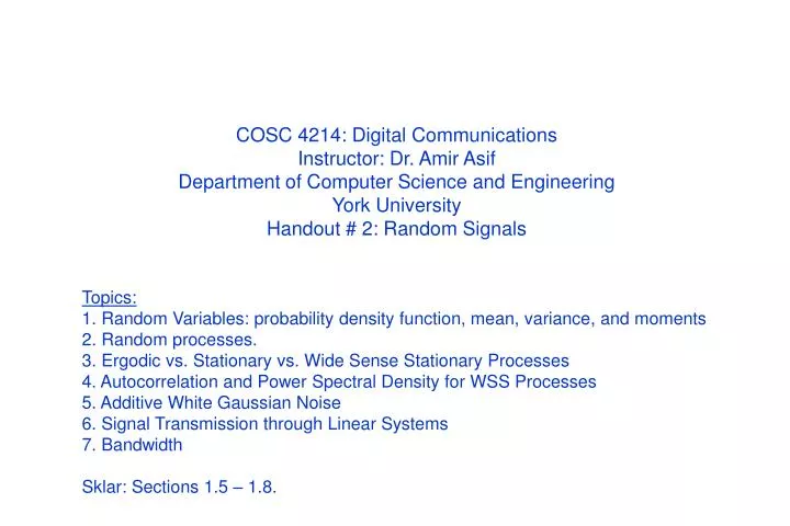
COSC 4214: Digital Communications Instructor: Dr. Amir Asif Department of Computer Science and Engineering York University Handout # 2: Random Signals Topics: 1. Random Variables: probability density function, mean, variance, and moments 2. Random processes.

E N D
COSC 4214: Digital Communications Instructor: Dr. Amir Asif Department of Computer Science and Engineering York University Handout # 2: Random Signals Topics: 1. Random Variables: probability density function, mean, variance, and moments 2. Random processes. 3. Ergodic vs. Stationary vs. Wide Sense Stationary Processes 4. Autocorrelation and Power Spectral Density for WSS Processes 5. Additive White Gaussian Noise 6. Signal Transmission through Linear Systems 7. Bandwidth Sklar: Sections 1.5 – 1.8.
Random Variables (1) Sample Space: is a set of all possible outcomes Example I: S = {HH, HT, TH, TT} in tossing of a coin twice. Example II: S = {NNN, NND, NDN, NDD, DNN, DND, DDN, DDD} in testing three electronic components with N denoting nondefective and D denoting defective. Random variable is a function that associates a real number with each outcome of an experiment. Example I: In tossing of a coin, we count the number of heads and call it the RV X Possible values ofX = 0, 1, 2. Example II: In testing of electronic components, we associate RV Yto the number of defective components. Possible values of Y = 0, 1, 2, 3. Discrete RV: takes discrete set of values. RV X and Y in above examples are discrete Continuous RV: takes values on an analog scale. Example III: Distance traveled by a car in 5 hours Example IV: Measured voltage across a resistor using an analog meter.
Random Variables (2) Probability density function of a discrete RV: is the distribution of probabilities for different values of the RV. Example I: S = {HH, HT, TH, TT} in tossing of a coin twice with X = no. of heads Example II: S = {NNN, NND, NDN, NDD, DNN, DND, DDN, DDD} in testing electronic components with Y = number of defective components. Properties:
pX(x) 0.01 X 150 250 Random Variables (3) Probability density function of a continuous RV: is represented as a continuous function of X. Example III: Distance traveled by a car in 5 hours has an uniform distribution between 150 and 250 km. Properties of pdf:
Random Variables (4) Activity 1: The pdf of a discrete RV X is given by the following table. Calculate the probability P(1 ≤ X < 3) and P(1 ≤ X ≤ 3) Activity 2: The pdf of a continuous RV X is pX(x) = e-xu(x). Find the probability P(1 < X < 5).
Random Variables (5) Distribution function: is defined as which gives Moments: Mean is defined as mX = E{X}.Variance is defined as var{X} = E{X}2 – (mX)2. Activity 3: Calculate and plot the distribution function for pdf’s specified in Activities 1 and 2. Also calculate the mean and variance in each case.
Random Processes (1) The outcome of a random process is a time varying function. Examples of ransom processes are: temperature of a room; output of an amplifier; or luminance of a bulb. A random process can also be thought of as a collection of RV’s for specified time instants. For example, X(tk), measured at t = tk is a RV.
Random Processes (2) Random processes are often specified by their mean and autocorrelation. Mean is defined as Autocorrelation is defined as Activity 4: Consider a random process where A and f0 are constants, while f is a uniformly distributed RV over (0, 2p). Calculate the mean and autocorrelation for the aforementioned process.
Random Processes WSS Stationary Ergodic Classification of Random Processes (1) Wide Sense Stationary (WSS) Process: A random process is said to be WSS if its mean and autocorrelation is not affected with a shift in the time origin Strict Sense Stationary (SSS) Process: A random process is said to be SSS if none of its statistics change with a shift in the time origin Ergodic Process: Time averages equal the statistical averages.
Classification of Random Processes (2) Activity 5: Show that the random process in Activity 4 is a WSS process. For WSS processes, the autocorrelation can be expressed as a function of single variable Autocorrelation satisfies the following properties Fourier transform of autocorrelation is referred to as the power spectral density (PSD)
Classification of Random Processes (3) Activity 6: Determine which of the following are valid autocorrelation function Activity 7: Determine which of the following are valid power spectral density function
Additive Gaussian Noise • Noise refers to unwanted interference that tends to obscure the information bearing signal • Noise can be classified into two categories: • Man-made Noise introduced by switching transients and simultaneous presence of neighboring signals • Natural Noise produced by the atmosphere, galactic sources, and heating up of electrical components. The latter is referred to as the thermal noise. • Thermal noise is difficult to be eliminated and often modeled by the Gaussian probability density function which has a mean mn= 0 and var(n) = s2.
Additive White Gaussian Noise Additive Gaussian Noise: refers to the following model for introduction of noise in the signal Given that the noise n is a Gaussian RV and a is the dc component, which is constant, the pdf of z is given by which has a mean mn= a and var(n) = s2. Additive White Gaussian Noise (AWGN): adds an additional constraint on the power spectral density Activity 8: Calculate the variance of AWGN given its PSD is N0/2.
Output Signaly(t) LTI Systemh(t) Input Signalx(t) Signal Processing with Linear Systems (1) • For deterministic signals, the output of the LTI system is given by • Convolution integral: • Transfer function: where X(f) and H(f) are Fourier transforms of x(t) and h(t). Activity 9: Determine the output of the LTI system if the input signal x(t) = e-atu(t) and the transfer function h(t) = e-btu(t) with a≠b.
Output Signaly(t) LTI Systemh(t) Input Signalx(t) Signal Processing with Linear Systems (2) For WSS random processes, statistics of the output of the LTI system can only be evaluated using the following formula. Activity 10: Derive the above expressions for WSS random processes. Activity 11: Calculate the mean and autocorrelation of the output of the LTI system if the input x(t) to the system is White Noise with PSD of N0/2 and the impulse response of the system is given byh(t) = e-btu(t).
Distortionless Transmission Communication System h(t) Output Signaly(t) Input Signalx(t) • For distortionless transmission, the signal can only undergo • Amplification or attenuation by a constant factor of K • Time delay of t0 In other words, there is no change in the shape of the signal • For distortionless transmission, the received signal must be given by • Based on the above model, the transfer function of the overall communication system is given by with impulse response
Ideal Filters Activity 12: Calculate the impulse response for each of the three ideal filters. Activity 13: Calculate the PSD and autocorrelation of the output of the LPF if WGN with PSD of N0/2 is applied at the input of the LPF.
1 t t 0 w 0 Bandwidth For baseband signals, absolute bandwidth is defined asthe difference between the maximum and minimum frequency present in a signal. Most time limited signals are not band limited so strictly speaking, their absolute bandwidth approaches infinity
Bandwidth for Bandpass signals(2) Alternate definitions of bandwidth include: Half-power Bandwidth: Interval between frequencies where PSD drops to 0.707 (3dB) of the peak value. Noise Equivalent Bandwidth is the ratio of the total signal power (Px) over all frequencies to the maximum value of PSD Gx(fc). Null to Null Bandwidth: is the width of the main spectral lobe. Fractional Power Containment Bandwidth: is the frequency band centered around fc containing 99% of the signal power
Bandwidth for Bandpass signals(3) Alternate definitions of bandwidth include: Bounded Power Spectral Density: the width of the band outside which the PSD has dropped to a certain specified level (35dB, 50dB) od the peak value. Absolute Bandwidth: Band outside which the PSD = 0.