Fourier Series

1. 1 Fourier Series Dr. K.W. Chow Mechanical Engineering

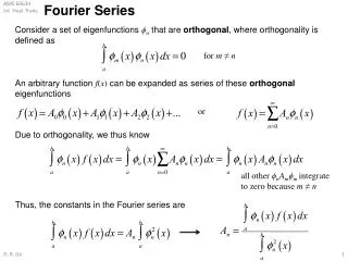
2. 2 Introduction Conceptual question: While one can readily see that two vectors can be �perpendicular� or �orthogonal�, how can we extend this concept to a sequence of functions?

3. 3 Introduction A general formulation: For a sequence of functions {fn} and f(x) = S cn fn What is cn ? IF ? fm fn dx = 0 for m, n different, then cn can be found from this �orthogonal� property.

4. 4 Introduction A general theory has been developed for linear, second order differential equations regarding these issues: (a) Orthogonal �eigenfunctions�? (b) Completeness in terms of expansion? (i.e. is it possible for any arbitrary function f(x) to be represented as a sum of fn(x)?)

5. 5 Introduction Sin(x) and Cos(x) are the solutions of the simplest second order ordinary differential equations (ODEs) d2y/dx2 + y = 0, subject to certain boundary conditions.

6. 6 Introduction Fourier series is an infinite series of sine and cosine Dirichlet�s theorem (Sufficient, but not necessary): If a function is 2L-periodic and piecewise continuous, then its Fourier series converges At a point of discontinuity, the series converges to the mean value.

7. 7 Fourier series an and bn are calculated by the orthogonal properties of sines and cosines. If one uses a0 as the constant term, two schemes for defining an, n = 0 and n > 0. If one uses a0/2, then one definition for all an .

8. 8 Introduction Consider:

9. 9

10. 10

11. 11

12. 12

13. 13 Introduction The n = 15 series gives a very good approximation to the original function

14. 14 Introduction

15. 15 Introduction Even extension of a function results in Fourier cosine series Odd extension of a function results in Fourier sine series (Assuming function is given only in half the interval.)

16. 16 Introduction

17. 17 Introduction

18. 18 Consider using odd extension

19. 19

20. 20

21. 21

22. 22

23. 23 Introduction

24. 24 Introduction

25. 25 Introduction

26. 26 Introduction

27. 27 Introduction

28. 28 Introduction Gibbs phenomenon � large oscillations of the series near a discontinuity.

29. 29 Introduction Consider the square wave again:

30. 30 Introduction

31. 31 Introduction

32. 32 Introduction Animation to show the Gibbs phenomenon using different partial sums.

33. 33 Differentiation of series Fourier coefficients are determined uniquely using orthogonality of trigonometric functions. only when the series on the right is uniformly convergent. (d/dx = a local operator)

34. 34 Integration of series Always permitted, but the resulting series is not a Fourier series, unless the constant term a0 is zero. (Integration = a global operator).

35. 35 1D heat conduction in finite domain Configuration:

36. 36 1D heat conduction in finite domain Thermal conductivity defined by Heat flux = - k A ?u/?x where A = cross sectional area, u = temperature (i.e. k is heat flux per unit area per unit temperature gradient).

37. 37 1D heat conduction in finite domain Assumptions: Heat flow in the x direction only No external heat source No heat loss

38. 38 1D heat conduction in finite domain Consider heat conduction across an infinitesimal element of the conductor:

39. 39 1D heat conduction in finite domain Heat flux at the left surface : - k A ?u(x,t)/?x Heat flux at the right surface: - k A ?u(x,t)/?x - ?[k A ?u(x,t)/?x]/?x dx + � Net heat flux INTO the element: ?[k A ?u(x,t)/?x]/?x dx

40. 40 1D heat conduction in finite domain Net heat must be used to heat up the element (c = specific heat capacity):

41. 41 1D heat conduction in finite domain Therefore (if k and A not functions of x):

42. 42 1D heat conduction in finite domain When , the above equation becomes exact: This is the 1D heat conduction equation in finite domain.

43. 43 1D heat conduction in finite domain Solution procedure Separation of variables: Substitute back into the heat equation:

44. 44 1D heat conduction in finite domain

45. 45 1D heat conduction in finite domain Assume both ends are kept at : For non-trivial solution, choose:

46. 46 1D heat conduction in finite domain F satisfies the differential equation: For non-trivial solutions: The temporal part:

47. 47 1D heat conduction in finite domain Overall solution: Using superposition principle, we obtain general solution:

48. 48 1D heat conduction in finite domain is the Fourier sine coefficient:

49. 49 1D heat conduction in finite domain is called the eigen-value is called the corresponding eigen-function

50. 50 1D heat conduction in finite domain Consider:

51. 51

52. 52

53. 53

54. 54

55. 55

56. 56

57. 57 1D heat conduction in finite domain The above procedure cannot be applied directly when the end points are not at First find steady-state temperature distribution v:

58. 58 1D heat conduction in finite domain Introduce a new function (transient): w satisfies the heat equation with homogeneous boundary conditions. Solve for w with separation of variables and hence u can be found.

59. 59 1D heat conduction in finite domain Consider:

60. 60

61. 61

62. 62

63. 63

64. 64

65. 65

66. 66 Laplace�s equation For heat conduction in higher dimensions, where is the Laplacian.

67. 67 Laplace�s equation The steady-state solution in 2D satisfies: which is the Laplace�s equation In the presence of heat sources, u satisfies the Poisson�s equation:

68. 68 Laplace�s equation 3 types of boundary conditions: Dirichlet boundary condition Neumann boundary condition Robin boundary condition

69. 69 Laplace�s equation Dirichlet boundary condition

70. 70 Laplace�s equation Neumann boundary condition

71. 71 Laplace�s equation Robin boundary condition

72. 72 Laplace�s equation Consider (Dirichlet b.c.)

73. 73 Laplace�s equation u(x, y) = F(x) G(y) F��/F = � G��/G = constant F(0) = F(a) = 0 and thus the constant is � n2 p 2 / L2 . Hence F ~ sin (n p x/L) G ~ cosh

74. 74 Laplace�s equation Solution is obtained using separation of variables:

75. 75 Laplace�s equation Consider

76. 76

77. 77

78. 78 1D wave equation in finite domain Configuration: Assumptions: - CONSTANT TENSION and density, - the slope of the vibration is small, - gravity much smaller than tension.

79. 79 1D wave equation in finite domain

80. 80 1D wave equation in finite domain Vertical force at the left end: Vertical force at the right end: u = u(x, t) = displacement of the string

81. 81 1D wave equation in finite domain Net vertical upward force on the element:

82. 82 1D wave equation in finite domain Newton�s second law (? = linear density):

83. 83 1D wave equation in finite domain When , the equation becomes exact. If no external force is present:

84. 84 1D wave equation in finite domain c = speed of the wave Check the dimensions: Square root of (force/mass per unit length). Mathematically, signs of two second derivatives same (contrast with Laplace equation).

85. 85 1D wave equation in finite domain Consider a vibrating string with two ends fixed and initial position and velocity given; i.e. initial and boundary conditions:

86. 86 Separation of Variables u(x, y) = F(x) G(t) F��/F = G��/(c2 G) = constant F(0) = F(a) = 0 and thus the constant is � n2 p 2 / L2 . Hence F ~ sin (n p x/L) G ~ C1sin (c n p t/L)+C2 cos (c n p t/L)

87. 87 1D wave equation in finite domain Solution obtained by separation of variables:

88. 88 1D wave equation in finite domain Modes of vibration are the profiles of the envelopes corresponding to different n

89. 89 1D wave equation in finite domain The mode shapes will oscillate with time

90. 90 1D wave equation in finite domain Another example � Vibration of a stretched string with a triangular initial profile. Qualitatively, the shapes of the string at subsequent times are similar to the n = 1 mode previously. However, the shapes remain piecewise linear, and some �corners� persist.

91. 91 1D wave equation in finite domain Consider:

92. 92 1D wave equation in finite domain

93. 93

94. 94

95. 95

96. 96

97. 97

98. 98

99. 99

100. 100

101. 101

102. 102

103. 103

104. 104

105. 105

106. 106 1D wave equation in finite domain General solution (d�Alembert) to the wave equation: Using trigonometric identities, the Fourier series solution can also be rewritten in the above form.

107. 107 1D wave equation in finite domain x- ct represents a wave traveling to the right with speed c

108. 108 1D wave equation in finite domain x + ct represents a wave traveling to the left with speed c

109. 109 1D wave equation in finite domain The lines are known as characteristic lines (or just characteristics). The forms of functions F and G depend on the initial conditions. The initial profile splits into two waves of same amplitude traveling in opposite directions

110. 110 1D wave equation in finite domain

111. 111 1D wave equation in finite domain Method of characteristics is of tremendous theoretical significance but less practical interest. Usually we just use separation of variables for finite domains and integral transform for infinite ones.

112. 112 PDEs in infinite domain Fourier series gives information in the interval Fourier series will give the periodic extension outside this domain. Fourier �fails� if the given function is already defined along the whole real-axis.

113. 113 From Fourier series to Fourier integrals To represent a function from minus infinity to plus infinity, we use a Fourier series over the interval (- L, L) and let L go to infinity. Result (Fourier integral): f = integral (integral f d?) dx

114. 114 From Fourier series to Fourier integrals f(x) = sum over An cos (n p x/L) An = 2/L integral f(?) cos (n p ?/L)d? Hence f(x) = sum over n [ 2/L (integral of f(?) cos (n p (x � ? )/L) d? ) ] Now convert �sum over n and (1/L)� into another integral.

115. 115 PDEs in infinite domain Separation of variables is usually not feasible or will fail. Use integral transforms: - Fourier transform - Laplace transform - �

116. 116 PDEs in infinite domain Fourier integrals are analogous to Fourier series:

117. 117 PDEs in infinite domain For functions defined in semi-infinite domain, even extension Fourier cosine integral odd extension Fourier sine integral

118. 118 PDEs in infinite domain Fourier transform pair:

119. 119 PDEs in infinite domain In some alternative versions, the + and - signs in the exponentials are interchanged. There is no universally accepted format. The constants in front of the integral signs are arbitrary, as long as their product is

120. 120 Applications of Fourier transform Idea: A PDE defined in an infinite domain is given. Apply transform on each term in the equation, with respect to a certain independent variable, e.g. x Derivatives in x become algebraic in ?.

121. 121 Applications of Fourier transform The transformed equation becomes an ODE in t (? is a parameter, no derivatives in ?), rather than PDE in x and t. Solve for the transformed function. Apply inverse transform to obtain solution in the original coordinates.

122. 122 Applications of Fourier transform Common techniques: Integration by parts Exchange order of integrations Contour integrals Gaussian integrals

123. 123 Applications of Fourier transform Example : heat equation Spatial conditions: u(x, t) decaying in far field. This represents an initially concentrated source of unit intensity at the origin

124. 124 Applications of Fourier transform

125. 125

126. 126

127. 127

128. 128

129. 129

130. 130

131. 131 This represents a uniform initial temperature distribution