Download
1 / 66
670 likes | 948 Views
Lecture 6. First order Circuits (i). Linear time-invariant first-order circuit, zero input response. The RC circuits. Charging capacitor Discharging capacitor The RL circuits. The zero-input response as a function of the initial state. Mechanical examples.

E N D
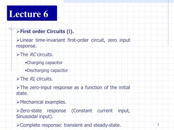
Lecture 6 • First order Circuits (i). • Linear time-invariant first-order circuit, zero input response. • The RC circuits. • Charging capacitor • Discharging capacitor • The RL circuits. • The zero-input response as a function of the initial state. • Mechanical examples. • Zero-state response (Constant current input, Sinusoidal input). • Complete response: transient and steady-state.
Why first order? In this lecture we shall analyze circuits with more than one kind of element; as a consequence, we shall have to use differentiation and/or integration. We shall restrict ourselves here to circuits that can be described by first-order differential equations; hence we give them the name first-order circuits
Linear Time –invariant First order Circuit. Zero-input Response TheRC Circuits In the circuit of Fig.6.1., the linear time-invariant capacitor with capacitance C is charged to a potential V0by a constant voltage source. At t=0 the switch k1is opened, and switch k2 is closed simultaneously. k2 k1 i(t) + v=V0 _ C E=V0 R Fig.6.1 A charged capacitor is connected to a resistor (k1, opens and k2closes at t=0).
Thus the charged capacitor is disconnected from the source and connected to the linear time-invariant resistor with resistanceRat t=0. Let us describe physically what is going to happen. Because of the charges stored in the capacitor(Q0=CV0)a current will flow in the direction specified by the reference direction assigned toi(t),as shown in Fig. 6.1. The charge across the capacitor will decrease gradually and eventually will become zero; the current i will do the same. During the process the electric energy stored in the capacitor is dissipated as heat in the resistor. Let us restricting our attention to t0, we redraw the RC circuit as shown in Fig.6.2. Note that the reference direction for branch voltages and branch currents are clearly indicated. V0 along with the positive and negative sins next to the capacitor, specifies the magnetite and polarity of the initial voltage. ic(t) iR(t) + + vR(t) - + vC(t) - vc(t)=V0 - Fig.6.2 An RC circuit, vc(0)=V0
Kirchoff`’s laws and topology dictate the following equations: (6.1) KVL: (6.2) KCL: The two branch equations for the two circuit elements are (6.3) Resistor: (6.4a) Capacitor: or, equivalently (6.4b) In Eq.(6.4a) we want to emphasize that the initial condition
Of the capacitor voltage must be written together with ; otherwise, the state of the capacitor is not completely specified. This is made obvious by the alternate branch equation (6.4b) Finally we have four equations for four unknown in the circuit, namely, the two branch voltages vC and vR and two branch currents iC and iR. A complete mathematical description of the circuit has been given and we can solve for any or all of the unknown parameters. If we wish to find the voltage across the capacitor, the combining Eqs (6.1) to (6.4a) we obtain for t0, (6.5)
This is a first-order linear homogeneous differential equation with constant coefficients. Its solution is of the exponential form (6.6) where (6.7) This easily verified by direct substitution of Eqs. (6.6) and (6.7) in the differential equation (6.5). In (6.6) K is a constant to be determined from the initial conditions. Setting t=0 in Eq.(6.6), we obtain vC(0)=K=V0. Therefore, the solution to the problem is given by (6.8)
vC V0 0.377V0 t 4T 0 T 2T 3T In Eq.(6.8), vC(t) is specified for t0 since for negative t the voltage across the capacitor is a constant, according to our original physical specification. The voltage vC(t) is plotted in Fig. 6.3 as a function of time. Of course, we can immediately the other three branch variables once vC(t) is known. From Eq.(6.4a) we have (6.9) From Eq.(6.2) we have (6.10) From Eq. (6.3) we have (6.11) Fig.6.3 The discharge of the Capacitor of Fig. 6.2 is given by an experimental curve
iC Exercise Show that the red line in Fig. 6.3, which is tangent to the curve vc(t)=0+, intersects the time axis at the abscissa T t 0 iR t vR Fig.6.4. Network variables iC ,iRand vR against time for t0. t
Let us study the waveform vc() more carefully. The voltage across the capacitor decreases exponentially with time, as shown in Fig. 6.3. An exponential curve can be characterized by two numbers, namely the ordinate of the curve at a reference time say t=0 and the time constant T which is defined by . In Fig. 6.3 we have f=V0 and T=RC. Remark The term s0=-1/T=-1/RC in Eqs.(6.6) and (6.7 has a dimension of reciprocal time of frequency and is measured in radians per second. It is called the natural frequency of the circuit. Exercise Recall that the unit of capacitance is the farad and the unit of resistance is the ohm. Show that the unit of T=RC is the second. In the circuit analysis we are almost always interested in the behavior of a particular network called the response. In general we give the name of zero-input response to the response of the circuit with no applied input
k2 A B k1 L R I0 The RL (Resistor –Inductor) Circuit The other typical first-order circuit is the RL circuit. We shall study its zero-input response. As shown in Fig. 6.5 for t<0, switch k1 is on terminal B, k2 is open, and the linear time-invariant inductor with inductance L is supplied with a constant current I0. At t=0 switch k1 is flipped to terminal C and k2 is closed. Thus for t0 the inductor with initial current I0 is connected to a linear time-invariant resistor with resistance R. The energy stored in the magnetic field as a result of I0 in the inductance decreases gradually and dissipate in the resistor in the form of heat. The current in the RL loop decreases monotonically and eventually tends to zero. Fig. 6.5.for t<0, switch k1 is on terminal B, k2 is open; therefore for t<0, the current I0 goes through the inductor L
In the same way as in RC case we redraw the RL circuit for t0 as shown in Fig.6.6. Note that the reference direction of all branch voltages and branch currents are clearly indicated. KCL says iR=-iL and KVL states vL-vR=0. Using the branch equations for both elements that is , , we obtain the following differential equation in terms of the current iL: + vL(t) - + vR - iL(0)=I0 iR (6.12) This is a first-order linear homogeneous differential equation with constant coefficients; it has precisely the same form as the previous Eq.6.5. Therefore the solution is the same except notations (6.13) where L/R=T is the time constant and s0=-R/L is the natural frequency Fig.6.6 An RL circuit with iL(0)=I0 and the waveforms for t0
The zero-input response as a function of the initial state For the RC circuit and the RL circuit considered above, the zero-input responses are respectively (6.14) The initial conditions are specified by V0 and I0, respectively. The numbers V0 and I0are also called the initial state of the RC circuit and of the RL circuit, respectively. The following conclusion could be reached if we consider the way in which the waveform of the zero-input response depends on the initial state. For first-order linear time invariant circuits, the zero-input response considered as a waveform defined for 0 t < is a linear function of the initial state Let us prove this statement by considering the RC circuit. We wish to show that the waveform v() in Eq. (6.14) is a linear function of the initial state V0. It is necessary to check the requirements of homogeneity and addittivity for the function.
Homogeneity is obvious; if the initial state is multiplied by a constant k, (Eq. (6.14)show that the whole waveform is multiplied by k. Adittivity as just as simple. The zero input response corresponding to the initial state V0’ is and the zero-input response corresponding to some other initial state V0” is Then the zero-input response corresponding to the initial state This waveform is the sum of the two preceding waveforms. Hence addittivity holds.
+ v - + vR - iR C=1 F Remark This property does not hold in the case of nonlinear circuits. Consider the RC circuit shown in Fig. 6.7a. The capacitor is linear and time invariant and has a capacitance of 1 farad, and the resistor is nonlinear with characteristic The two elements have the same voltage v, and expressing the branch currents in terms of v, we obtain from KCL Hence If we integrate between 0 an t, the voltage takes the initial value V0 and the final value v(t); hence Fig.6.7a Nonlinear RC circuit and two of its zero-input resistance. The capacitor is linear and the resistor
or (6.15) This is the zero-input response of this nonlinear RC circuit starting from the initial state V0 at time 0. The waveforms corresponding to V0=0.5and V0=2 are plotted in Fig 6.7b. v It is obvious that the top curve (V0=2) cannot be obtained from the lower one (for V0=0.5) by multiplying its ordinates by 4. 2.0 1.5 V0=2 1.0 0.5 V0=0.5 Fig. 6.7b t
v(t) v(0)=V0 M Bv (friction forces) Mechanical example Let us consider a familiar mechanical system that has a behavior similar to that of the linear time invariant RC and RL circuits above. Figure 6.8 shows a block of mass M moving at an initial velocity V0at t=0. Fig. 6.8 A mechanical system which is described by a first order differential equation As time proceeds, the block will slow down gradually because friction tends to oppose the motion. Friction is represented by friction forces that are all ways in the direction opposite to the velocity v, as shown in the figure. Let us assume that these forces are proportional to the magnitude of the velocity; thus, f=Bv, where the constant B is called the damping coefficient. From Newton’s second law of motion we have, for t0,
(6.16) Therefore (6.17) where M/B represents the time constant for the mechanical system and –B/M is the natural frequency
C R is(t)=I k Zero-state Response Constant Current Input In the circuit of Fig. 6.9 a current source is is switched to a parallel linear time invariant RC circuit. For simplicity we consider first the case when the current is is constant and equal to I. Prior to the opening of the switch the current source produces a circulating current in the short circuit. At t =0, the switch is opened and thus the current source is connected the RC circuit. From KVL we see that the voltage across all three elements is the same. Let us design this voltage by v and assume that v is the response of interest. Writing the KCL equation in terms of v, we obtain the following network equation: Fig.6.9 RC circuit with current source input. At t=0, switch k is opned
(6.18) where I is a constant. Let us assume that the capacitor is initially uncharged. Thus, the initial condition is (6.19) Before we solve Eqs. (6.18) and (6.19), let s figure out what will happen after we open the switch. At t=0+, that is, immediately after the opening of the switch, the voltage across the capacitor remains zero, because as we learned the voltage across a capacitor cannot jump abruptly unless there is an infinitely large current. At t=0+, since the voltage is still zero, the current in the resistor must be zero by Ohm’s law. Therefore all the current from the source enters the capacitor at t=0+. Thus implies a rate of increase of the voltage specified by Eq.(6.19), thus (6.20)
v RI t As time proceeds, v increases, and v/R, the current through the resistor, increases also. Long after the switch is opened the capacitor is completely charged, and the voltage is practically constant. Then and thereafter, dv/dt0. All the current from the source goes through the resistor, and the capacitor behaves as an open circuit, that is (6.21) This fact is clear form Eq.(6.18), and it is also shown in Fig.6.10. The circuit is said to have reached a steady state. It only remains to show how the whole change of voltage takes place. For that we rely on the following analytical treatment. The solution of a linear no homogeneous differential equation can be written in the following form: (6.22) Fig. 6.10. Initial and final behavior of the voltage across the capacitor.
where vh is a solution of the homogeneous differential equation and vp is any particular solution of the nonhomogenous differential equation. vp depends on the input. The general solution of the homogeneous equation is of the form (6.23) where K1 is any constant. The most convenient particular solution for a constant current input is a constant (6.24) since the constant RI satisfies the differential equation (6.18). Substituting (6.23) and (6.24) in (6.22), we obtain the general solution of (6.18) (6.25) where K1 is to be evaluated from the initial condition specified by Eq.(6.19). Setting t=0 in (6.25), we have
v RI t Thus, (6.26) The volt age as a function of time is then (6.27) The graph in Fig.6.11 shows the voltage approaching its steady-state value exponentially. At about four times the time constant, the voltage is with two percent of its final value RI 0.05RI 0.02RI 0.63 RI 3T 4T T 2T Fig. 6.11. Voltage response for the RC circuit due to a constant source Ias shown in Fig. 6.10 wherev=0
Exercise 1 Sketch with appropriate scales the zero state response of the of Fig.6.10 with • I=200 mA, R=1 k, and C=1F • I=2 mA, R=50 , and C=5 nF Exercise 2 • Calculate and sketch the waveforms ps() (the power delivered by the source), pR() (the power dissipated by the resistor) and EC(), (the energy stored in the capacitor) • Calculate the efficiency of the process, i.e the ratio of the energy eventually stored in the capacitor to the energy delivered by the source [ ]
Sinusoidal Input We consider now the same circuit but with a different input; the source is now given by a sinusoid (6.28) where the constant A1 is called the amplitude of the sinusoids and the constant is called the (angular) frequency. The frequency is measure in radians per second. The constant 1 is called phase. The solution of the homogeneous differential equation if of the same form (See Eq.(6.23)), since the circuit is the same except input. The most convenient particular solution of a linear differential equation with a constant coefficient for a sinusoidal input is a sinusoid of the same frequency. Thus vpis taken to be of the form (6.29) where A2 and 2 are constants to be determined. To evaluate them , we substitute (6.29) in the given differential equation, namely
Using standard trigonometric identities to express , and and and as a linear combination of and we obtain equating separately the coefficients of the following results: (6.30) We obtain (6.31) (6.32) and (6.33)
is A1 t A2 t1 t Here tan-1RC denotes the angle between 0 and 90o whose tangent is equal to RC . This particular solution and the input current are plotted in Fig. 6.12. Fig.6.12 Input current and a particular solution for the output voltage of the RC circuit in Fig.6.9. vp
Exercise Derive Eqs. (6.32) and (6.33) in detail. The general solution of (6.31) is therefore of the form (6.34) Setting t=0, we have (6.35) that is (6.36) Therefore the response is given by (6.37) where A2and 2 are defined in Eqs.(6.32) and (6.33). The graph of v, that is the zero-state response to the input A1 cos(t+1), is plotted in Fig.6.13.
v vp v(t) t vh Fig.6.13. Voltage response of the circuit in Fig. 6.13 with v(0)=0 and is(t)=A1cos(t+1) In the two cases treated in this lecture we considered the voltage v as the response and the current source isas the input. The initial condition in the circuit is zero; that is, the voltage across the capacitor is zero before the application of the input. In general we say that a circuit is in the zero state is all the initial conditions in the circuit are zero. The response of a circuit which starts from the zero state, is due exclusively to the input. By definition, the zero-state response is the response of a circuit to an input applied at some arbitrary time, say, t0, subject to the condition that the circuit be in the zero state just prior to the application of the input (that is, at time t0-). In calculating zero-state responses, our primary interest is the behavior of the response for tt0. It means that the input and the zero-state response are taken to be identically zero at t<t0.
B + k + A C V0 v R is(t) - - Complete Response: Transient and Steady state Complete response. The response of the circuit to both an input and the initial conditions is called the complete response of the circuit. Thus the zero-input response and the zero-state response are special cases of the complete response. Let us demonstrate that for the simple linear RC circuit considered, the complete response is the sum of the zero-input response and the zero-state response. Consider the circuit in Fig. 6.14 where the capacitor is initially charged; that isv(0)=V00, and a current input is switched into the circuit at t=0. Fig.6.14 RC circuit with v(0)=V0 is excited by a current source is(t).The switch k is flipped from A to B at t=0.
By definition, the complete response is the waveform v() caused by both the input and the initial is()state V0. (6.38) with (6.39) Where V0 is the initial voltage of the capacitor. Let vi be the zero-input response; by definition, it is the solution of with Let v0 be the zero-state response; by definition, it is the solution of with
From these four equations we obtain, by addition and However these two equations show that the waveform vi()+v0() satisfies both the required differential equation (6.38) and the initial condition (6.39). Since the solution of a differential equation such as (6.38), subject to initial conditions such as (6.39), is unique, it follows that the complete response v is given by that is, the complete response v is the sum of the zero-input response vi and the zero-state response v0.
Example If we assume that the input is a constant current source applied at t=0, that is, is=I, the complete response of the current can be written immediately since we have already calculated the zero-input response and the zero-state response. Thus, From Eq.(6.8) we have And from Eq.(6.27) we have Thus the complete response is (6.40) Complete response Zero-input Response vi Zero-state Response v0 The responses are shown in Fig.(6.15)
Remark We shall prove later that for the linear time invariant parallel RC circuit the complete response can be explicitly written in the following form for any arbitrary input is: Complete response Zero-input Response Zero-state Response Exercise By direct substitution show that the expression for the complete response given in the remark satisfies (6.38) and (6.39) v RI v0 vi t Fig.6.15 Zero-input, zero state and complete response of the simple RC circuit. The input is a constant current source I applied at t=0.
Transient and steady state. In the previous example we can also partition the complete response in a different way. The complete response due to the initial state V0 and the constant current input I in Eq.(6.40) 9s rewritten as follows (6.41) Complete response Steady state Transient The first term is a decaying exponential as represented by the shaded area, i.e., the difference of the waveform v() and the constant RI in Fig.6.15. For very large t, the first term is negligible, and the second term dominates. For this reason we call the first term the transient and the second term the steady state. In this example it is evident that transient is contributed by both the zero-input response and the zero-state response, whereas the steady sate is contributed only by the zero-state response. Physically, the transient is a result of two cases, namely, the initial conditions in the circuit and a sudden application of the input.
+ 1F v -1 is - The steady state is a result of only the input and has a waveform closely related to that of the input. If the input, for example, is a constant, the steady state response is also a constant; if the input is a sinusoid of angular frequency , the steady state response is also a sinusoid of the same frequency. In the example of sinusoid inpput, the input is ,the response has a steady state and a transient portion portion Exercise The circuit shown in Fig. 6.16 contains 1-farad linear capacitor and a linear resistor with a negative resistance. When the current source is applied, it is in the zero state at time t=0, so that for t0, is=Imcost. Calculate and sketch the response v. Is there a sinusoidal steady state? Fig.6.16 Exercise on steady state.
k2 + R2 C R1 I v k1 - Circuits with Two Time Constants Problems involving the calculation of transients occur frequently in circuits with switches. Let us illustrate such a problem with the circuit shown in Fig. 6.17. Assume that the capacitor and resistors are linear and time invariant, and that the capacitor is initially uncharged. For t<0 switch k1 is closed and switch k2 is open. Switch k1is opened at t=0 and thus connects the constant current source to the parallel RC circuit. The capacitor is gradually charged with the time constant T1=R1C1. Suppose that t=T1 ,switch k2 is closed. The problem is to determine the voltage waveform across the capacitor for t0. We can divide the problem into to parts, the interval [0,T1] and the interval [T1, ]. First we determine the voltage in [0,T1] before switch k2 closes. Fig.6.17 A simple transient problem. The switch k1 is opened at t=0; the switch k2 is closed at t=T1=R1C1.
Since v(0)=0 by assumption, the zero-state response can be found immediately. Thus, (6.42) At t=T1 (6.43) Which represents the initial condition for the second part of our problem. For t>T1 , since switch k2is closed we have a parallel combination of C, R1 and R2; the time constant is (6.44) and the input is I. The complete response for this second part is, for tT1. (6.45)
v R1I Time constant T1 Time constant T2 0 T1 t Fig.6.18 Waveform of voltage for the circuit in Fig.6.17.
I I I a I a R R b b + + C C e - - e RC Circuits RC 2RC Ce RC 2RC Ce q q 0 0 t t
Calculate Charging of Capacitor through a Resistor • Calculate Discharging of Capacitor through a Resistor
Last time--Behavior of Capacitors • Charging • Initially, the capacitor behaves like a wire. • After a long time, the capacitor behaves like an open • switch. • Discharging • Initially, the capacitor behaves like a battery. • After a long time, the capacitor behaves like a wire.
The capacitor is initially uncharged, and the two switches are open. E 3) What is the voltage across the capacitor immediately after switch S1 is closed? a) Vc = 0 b) Vc = E c) Vc = 1/2 E 4) Find the voltage across the capacitor after the switch has been closed for a very long time. a) Vc = 0 b) Vc = E c) Vc = 1/2 E
Initially:Q = 0 VC = 0 I = E/(2R) After a long time: VC = EQ = E C I = 0
Preflight 11: E 6) After being closed a long time, switch 1 is opened and switch 2 is closed. What is the current through the right resistor immediately after the switch 2 is closed? a) IR= 0 b) IR=E/(3R) c) IR=E/(2R) d) IR=E/R
After C is fully charged, S1 is opened and S2 is closed. Now, the battery and the resistor 2R are disconnected from the circuit. So we now have a different circuit. Since C is fully charged, VC = E. Initially, C acts like a battery, and I = VC/R.
I I a R b C e Would it matter where R is placed in the loop?? RC Circuits(Time-varying currents) • Charge capacitor: • Cinitially uncharged; connect switch toaat t=0 Calculate current and charge as function of time. • • Loop theorem Þ • Convert to differential equation for Q: No!
I I a R b C e Note that this “guess” incorporates the boundary conditions: ! RC Circuits(Time-varying currents) • Charge capacitor: • • Guess solution: • Check that it is a solution:
I • Charge capacitor: I a R b C e Þ • Conclusion: • Capacitor reaches its final charge(Q=Ce ) exponentially with time constant t = RC. • Current decays from max (=e /R) with same time constant. RC Circuits(Time-varying currents) • Current is found from differentiation:
Charge on C Max = Ce 63% Max at t=RC Current Max =e /R 37% Max at t=RC Charging Capacitor RC 2RC Ce Q 0 t e /R I 0 t