Download
1 / 31
320 likes | 469 Views
We shall now look at a second application of multi-bond graphs: 3D mechanics . 3D mechanical models look superficially just like planar mechanical models. There are additional types of joints, but other than that, there seem to be few surprises.

E N D
We shall now look at a second application of multi-bond graphs: 3D mechanics. 3D mechanical models look superficially just like planar mechanical models. There are additional types of joints, but other than that, there seem to be few surprises. Yet, the seemingly similar appearance is deceiving. There are a substantial number of complications that the modeler has to cope with when dealing with 3D mechanics. These are the subject of this lecture. 3D Mechanics
Degrees of freedom 3D mechanical multi-bonds 3D mechanical connectors Body-fixed coordinate system Orientation matrix Coordinate transformations Efficient simulation equations Computation of orientation matrix Quaternions Table of Contents • Wrapper models • Equations of motion • Eulerian Junction Structure • Model of a body
1D mechanical systems exhibit exactly one degree of freedom (either translational or rotational). 2D mechanical systems have three degrees of freedom. They can translate along two axes, and they can rotate around an axis that is perpendicular to the plane spanned by the two translational axes. 3D mechanical systems allow six degrees of freedom. They can translate along three spatial axes, and they can rotate around each of those three axes as well. Degrees of Freedom
Consequently, the 3D mechanical multi-bonds are expected to contain six parallel regular bonds, one for each degree of freedom: fy vy } fx f6 v vx fz vz tx x ty y tz z 3D Mechanical Multi-bonds Composition of a multi-bond for 3D mechanics
The 3D mechanical multi-bond connectors should carry 13 variables, an effort vector, e, of length 6, a flow vector, f, also of length 6, plus the directional variable, d. The 3D mechanical multi-body connectors would need to carry 18 variables, namely 12 potential variables describing the 6 generalized positions and the 6 generalized velocities, and 6 flow variables describing the generalized forces. In reality, they carry 24 variables, as shown on the next slide. 3D Mechanical Connectors
The orientation matrix R rotates the axes of the world model into the axes accompanying the body. Orientation of the axes in the body coordinate system. Orientation of the axes in the world coordinate system. 3D Mechanical Connectors II ωbody = R · ω0
In 3D mechanics, the inertial tensor depends on the orientation of the body relative to its coordinate system. Hence, if the world coordinate system is being used for formulating the d’Alembert principle for rotational motion, the inertial tensor must be constantly updated. Alternatively, we can formulate the d’Alembert principle in a body-fixed coordinate system. In this way, the inertial tensor remains constant. However, we now must calculate the relative coordinate transformations across joints. We must also take into account the gyroscopic torques that result from formulating the d’Alembert principle in an accelerated frame. The Body-fixed Coordinate System
In planar mechanics, this wasn’t a problem yet. There is a single axis of rotation that is always perpendicular to the plane of translation. Consequently, the inertia remains constant, and we can (and have been) calculating all motions in the world coordinate system. This fact makes planar mechanics considerably simpler and more easy to understand than 3D mechanics. The Body-fixed Coordinate System II
The orientation matrix, R, is a unitary matrix. Hence: Each row vector and each column vector of R is of length 1, hence there are 6 constraint equations connecting the 9 matrix elements. As expected, there are only 3 degrees of freedom, describing the relative rotation of one coordinate system to another. The Orientation Matrix ||R||2 = 1 R-1 = RT
Coordinate transformations can be interpreted as an act of transformation in a bond graph sense: τ1 = RT· τ2 Coordinate Transformations ω2 = R · ω1
We must separately also transform the angular positions: φ2 = Rrel· φ1 R2 = Rrel· R1 Coordinate Transformations II ω2 = Rrel· ω1
Dymola doesn’t understand the concept of a unitary matrix. Hence, if the computational causality requires an inversion of the R matrix, that is what Dymola will provide … in symbolic form. This leads to highly inefficient equations at run time. Thus, it is better to help Dymola by specifying the direction of computational flow explicitly. R1 = Rrel-1· R2 = RrelT· R2 Efficient Simulation Equations R2 = Rrel· R1
One way to compute the orientation matrix, R, in a non-redundant fashion is by means of Cardan angles. These are the angles of rotation around the Carthesian coordinates: φx, φy, and φz. R = Rz· Ry · Rx Computation of Orientation Matrix • Whereas R can always be computed out of φx , φy, and φz in a unique fashion, the opposite is unfortunately not true. • If φy = 90o, the other two axes are aligned, and φxand φzcannot be determined in a unique fashion. • Hence Cardan angles are not always a good choice.
~ 0 -n3 n2 n3 0 -n1 -n2 n1 0 (a × b = A · b) Ñ = Computation of Orientation Matrix III • Any 3D rotation can be expressed as a planar rotation, φ, perpendicular to a translational plane, n. • Given the rotation angle, φ, and the translational plane, n, the orientation matrix can be computed as follows: • where: R = n·nT+ (I - n·nT)cos(φ) – Ñsin(φ)
R = n·nT+ (I - n·nT)cos(φ) – Ñsin(φ) Computation of Orientation Matrix IV • Unfortunately, also the planar rotation method is not always invertible in a unique fashion. A null rotation does not have a well defined axis of rotation. Hence, this method should only be used if the axis of rotation is always known, as in a revolute joint.
Quaternions • A redundant way of describing orientation that works in all situations is by means of quaternions. • Quaternions are a four-dimensional extension to complex numbers: • Quaternions are characterized by the three imaginary components, i, j, and k that satisfy the following computational rules: Q = c + ui + vj + wk = c + u ij = k; ji = -k; i2 = -1 jk = i; kj = -i; j2 = -1 ki = j; ik = -j; k2 = -1
Q = c + u = c – u Quaternions II • The product of two quaternions can be written as: • The complement of a quaternion is being defined as: • The norm of a quaternion is the product of the quaternion with its complement: • A unit quaternion is a quaternion with norm 1: QQ’ = (c + u)(c’ + u’) = (cc’ – u·u’) + (u×u’) + cu’ + c’u QQ = | Q | = c2 + |u|2 | Q | = c2 + |u|2 = 1
~ R = 2u·uT+ 2cU +2c2I - I Quaternions III • In accordance with trigonometry: • it is always possible to find an angle φ such that: • This enables us to encode the orientation of a coordinate system as a quaternion, whereby the axis of rotation is encoded as u, where [u,v,w]T is being interpreted as a vector pointing in the direction of the axis of rotation. The fourth quantity, c, of the quaternion encodes the angle of rotation, φ. • Then: cos(φ/2)2 + sin(φ/2)2 = 1 c = cos(φ/2); |u| = sin(φ/2)
~ R = 2u·uT+ 2cU +2c2I - I Computation of Orientation Matrix V • The multi-bond graph library uses all three representations. It uses the planar rotation method inside revolute joints, and either Cardan angles or quaternions (user’s choice) within more general joints, such as the spherical joints.
Translational positions Rotational positions The Wrapper Models • In the multi-bond graph library, the equations of motion are formulated in the world coordinate system for translational motions, and in a body-fixed coordinate system for rotational motions. • For this reason, the bond graphs for translational and rotational motions are kept separate from each other, and the 3D mechanics multi-bonds have therefore still a cardinality of 3. Translational multi-bond graph Rotational multi-bond graph
. τ0 = J0 · ω0 ( ) RTJbodyωbody τ0 = . . d τ0 = RTJbodyωbody + RTJbodyωbody dt { τbody = Jbodyzbody + ωbody× Jbodyωbody Gyroscopic torque Equations of Motion in Body System • Let us formulate the equations of motion in a body-fixed coordinate system: ~ RTτbody = RTJbodyzbody + RTΩbodyJbodyωbody
The Eulerian Junction Structure • The gyroscopic torque can be formulated, in terms of bond graphs, as a so-called Eulerian Junction Structure (EJS): External description Multi-bond graph implementation Bond graph description
fwld = mawld - mgwld Translation Rotation τbdy = Jbdyzbdy + ωbdy × Jbdyωbdy The Model of a Body • We are now ready to model a general body using the multi-bond graph library: • The translational equations of motion are formulated in world coordinates. • The rotational equations of motion are formulated in body-fixed coordinates. • The gravitational pool is computed by the world model of wrapped 3D mechanics.
} General parameters } Parameters grouped into separate list on main parameter window Final parameters are computed parameters. They are not listed. The Model of a Body II
Parameters grouped into separate sub-windows of the general parameter window } The Model of a Body III
The Model of a Body IV • Every 3D mechanical wrapped multi-bond graph model must invoke the world3D model that must be declared in each wrapped multi-bond graph component model as an outer model.
The Model of a Body V • The shapes and sizes of bodies can be declared for the purpose of animation. • This feature is borrowed from the multi-body systems sub-library of the standard Modelica mechanics library. • You find documentation there for predefined shapes under the sub-heading Visualizers, and more generally under the sub-sub-entry of Advanced → Shape.
The Model of a Body VI • The center of the gravitational pool is specified in the equation window. The corresponding graphical element is only a drawing. The user is reminded of this fact, by not connecting the “connections” all the way to the connectors. The user then knows that “something is fishy.”
Zimmer, D. (2006),A Modelica Library for MultiBond Graphs and its Application in 3D-Mechanics, MS Thesis, Dept. of Computer Science, ETH Zurich. Zimmer, D. and F.E. Cellier (2006), “The Modelica Multi-bond Graph Library,” Proc. 5th Intl. Modelica Conference, Vienna, Austria, Vol.2, pp. 559-568. References I
Cellier, F.E. and D. Zimmer (2006), “Wrapping Multi-bond Graphs: A Structured Approach to Modeling Complex Multi-body Dynamics,” Proc. 20th European Conference on Modeling and Simulation, Bonn, Germany, pp. 7-13. References II