Download
1 / 20
200 likes | 304 Views
Ch. 8 Multiple Regression (con’t). Topics: F-tests : allow us to test joint hypotheses tests (tests involving one or more coefficients). Model Specification:

E N D
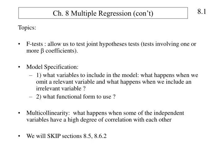
Ch. 8 Multiple Regression (con’t) Topics: • F-tests : allow us to test joint hypotheses tests (tests involving one or more coefficients). • Model Specification: • 1) what variables to include in the model: what happens when we omit a relevant variable and what happens when we include an irrelevant variable ? • 2) what functional form to use ? • Multicollinearity: what happens when some of the independent variables have a high degree of correlation with each other • We will SKIP sections 8.5, 8.6.2
F-tests • Previously we conducted hypothesis tests on individual coefficients using a t-test. • New Approach is the F-test: it is based on a comparison of the sum of squared residuals under the assumption that the null hypothesis is true and then under the assumption that it is false. • It is more general than the t-test because we can use it to test several coefficients jointly • Unrestricted model is: • Restricted model is something like: or
Types of Hypotheses that can be tested with a F-Test A. One of the ’s is zero. When we remove independent variables from the model, we are restricting its coefficient to be zero. Unrestricted: Restricted: We already know how to conduct this test using T-test. However, we could also test it with an F-test. Both tests should come to the same conclusion regarding Ho. Ho: 4 = 0 H1: 4 0
B. A Proper Subset of the Slope Coefficients are restricted to be zero: Unrestricted Model: Restricted: Ho : 3 = 4 = 0 H1: at least one of 3 , 4 is non-zero
C. All of the Slope Coefficients are restricted to be zero: U: R: Ho: 2 = 3 = 4 = 0 H1: at least one of 2 ,3 , 4 is non-zero We call this a test of overall model significance. If we fail to reject Ho our model has explained nothing. If we reject Ho our model has explained something.
Let SSER be the sum of squared residuals from the Restricted Model Let SSEU be the sum of squared residuals from the Unrestricted Model. Let J be the number of “restrictions” that are placed on the Unrestricted model in constructing the Restricted model. Let T be the number of observations in the data set. Let k be the number of RHS variables plus one for intercept in the Unrestricted model. Recall from Chapter 7 that the sum of squared residuals (SSE) for the model with fewer independent variables is always greater than or equal to the sum of squared residuals for the model with more independent variables. F-statistic has 2 measures of degrees of freedom: J in the numerator and T-k in the denominator
Critical F: use table on page 391 (5%) or 392 (1%) • Suppose J=1 and T=30 and k=3 • Critical F at 5% level of significance is Fc = 4.21 (see page 391), meaning P(F > 4.21) = 0.05 0.05 0 Fc F We calculate our F statistic using this formula: If F > Fc we reject null Hypothesis Ho If F < Fc we fail to reject Ho Note: F can never be negative
Airline Cost Function: Double Log model. See page 197, 8.14 The SAS System The REG Procedure Model: MODEL1 Dependent Variable: lvc Analysis of Variance Sum of Mean Source DF Squares Square F Value Pr > F Model 6 340.55467 56.75911 4110.31 <.0001 Error 261 3.60414 0.01381 Corrected Total 267 344.15881 Root MSE 0.11751 R-Square 0.9895 Dependent Mean 6.24382 Adj R-Sq 0.9893 Coeff Var 1.88205 Parameter Estimates Parameter Standard Variable DF Estimate Error t Value Pr > |t| Intercept 1 7.52890 0.58217 12.93 <.0001 ly 1 0.67916 0.05340 12.72 <.0001 lk 1 0.35031 0.05288 6.62 <.0001 lpl 1 0.27537 0.04381 6.29 <.0001 lpm 1 -0.06832 0.10034 -0.68 0.4966 lpf 1 0.32186 0.03610 8.92 <.0001 lstage 1 -0.19439 0.02858 -6.80 <.0001 SST SSEU
Jointly Test a proper subset of slope coefficients: Ho : 4 = 5 = 6 = 0 H1: at least one of 5 , 6 , 7 is non-zero SSER The REG Procedure Model: MODEL2 Dependent Variable: lvc Analysis of Variance Sum of Mean Source DF Squares Square F Value Pr > F Model 3 314.54167 104.84722 934.58 <.0001 Error 264 29.61714 0.11219 Corrected Total 267 344.15881 Root MSE 0.33494 R-Square 0.9139 Dependent Mean 6.24382 Adj R-Sq 0.9130 Coeff Var 5.36438 Parameter Estimates Parameter Standard Variable DF Estimate Error t Value Pr > |t| Intercept 1 5.78966 0.42629 13.58 <.0001 ly 1 0.76485 0.15123 5.06 <.0001 lk 1 0.24829 0.15022 1.65 0.0996 lstage 1 -0.02162 0.08037 -0.27 0.7881 Conduct the test
Test a single slope coefficient Ho : 4 = 0 H1: 4 0 SSER Dependent Variable: lvc Analysis of Variance Sum of Mean Source DF Squares Square F Value Pr > F Model 5 340.54827 68.10965 4942.40 <.0001 Error 262 3.61054 0.01378 Corrected Total 267 344.15881 Root MSE 0.11739 R-Square 0.9895 Dependent Mean 6.24382 Adj R-Sq 0.9893 Coeff Var 1.88012 Parameter Estimates Parameter Standard Variable DF Estimate Error t Value Pr > |t| Intercept 1 7.14687 0.15511 46.07 <.0001 ly 1 0.67669 0.05322 12.71 <.0001 lk 1 0.35230 0.05274 6.68 <.0001 lpl 1 0.26072 0.03812 6.84 <.0001 lpf 1 0.30199 0.02121 14.24 <.0001 lstage 1 -0.19368 0.02853 -6.79 <.0001 Conduct the test
Jointly test all of the slope coefficients To conduct the test that all the slope coefficients are zero, we do not estimate a restricted version of the model, because the restricted model has no independent variables on the right hand side. Ho: 2 = 3 = 4 = 5 = 6 = 7 = 0 H1: at least one of is non-zero. The restricted model explains none on the variation in the dependent variable. The SSRR is 0, meaning the unexplained portion is everything!! SSER = SST. (SST is the same for Unrestricted and Restricted Models.) Conduct the test:
Additional Hypothesis Tests EXAMPLE: trt = 1 + 2 pt + 3 at + 4 a2t + e This model suggests that the effect of advertising (at) on total revenues (trt) is nonlinear, specifically, it is quadratic. • If we want to test the hypothesis that advertising has any effect on total revenues, then we would test Ho: 3 = 4 =0; H1: at least one is nonzero. We would conduct the test using an F test. 2) If we want to test (instead of assuming) that the effect of advertising on total revenues is quadratic, as opposed to linear we would test the hypothesis Ho : 4 =0 ;H1: 4 0 . We could conduct this test using the F-test or a simple t-test (the t-test is easier because we estimate only on model instead of two).
Model Specification 1) Functional Form (Chapter 6) • Omitted Variables: the exclusion of a variables that belongs in the model. Is there a problem? Aside from not being able to get an estimate of 3, is there any problem with getting an estimate of 2? True Model: The Model We Estimate: We should have used this Formula B: We use this Formula A:
It can be shown that E(b2) 2, meaning that using Formula A (the bivariate formula for least squares) to estimate 2 results in a biased estimate when the true model is multiple regression (Formula B should have been used). In Ch. 4, we derived E(b2). Here it is:
Recap: When b2 is calculated using formula A (which assumes that x2 is the only independent variable) when the true model is that yt is determined by x2 and x3, then least squares willbe biased: E(b2) ≠ β2 So……not only do we not get an estimate of 3 (the effect of x3 on y), Our estimate of 2 (the effect of x2on y) is biased. Recall that Assumption 5 implies that independent variables in regression model are uncorrelated with the error term. When we omit an independent Variable, it is “thrown” into the error term. If the omitted variable is correlated with the included independent variables, this assumption 5 is violated and Least Squares is no longer an unbiased estimator. However, if x2 and x3 are uncorrelated b2 is unbiased. In general, the signs of 3 and Cov(x2,x3) determine the direction of the bias. Bias
Example of Omitted Variable Bias: True Model: The Model We Estimate: Our estimated model using annual data for U.S. Economy 1959-99: A corrected model
Inclusion of Irrelevant Variables: • This error is not nearly as severe as omitting a relevant variable. The Model We Estimate: True Model: • In truth 3 = 0, so our estimate b3 should be not be statistically different • from zero. The only problem is the Var(b2) will be larger than it should be • Results may appear to be less significant. Remove x3from the model and we should see a decrease in se(b2). The formula we should use: The formula we do use:
Multicollinearity • Economic data are usually from an uncontrolled experiment. Many of the economic variables move together in systematic ways. Variables are collinear, and the problem is labeled collinearity, or multicollinearity when several variables are involved. • Consider a production relationship: certain factors of production, such as labor and capital, are used in relatively fixed proportions Proportionate relationships between variables are the very sort of systematic relationships that epitomize “collinearity.” • A related problem exists when the values of an explanatory variable do not vary or change much within the sample of data. When an explanatory variable exhibits little variation, then it is difficult to isolate its impact. • We generally always have some of it. It is a matter or degree.
The Statistical Consequences of Collinearity • Whenever there are one or more exact linear relationships among the explanatory variables exact (perfect) multicollinearity. Least squares is not defined; can’t identify the separate effects. • When nearly exact linear dependencies (high correlations) among the X’s exist, the variances of the least squares estimators may be large least square estimator will lack precision small t-statistics (insignificant results), despite possibly high R2 or “F-values” indicating “significant” explanatory power of the model as a whole. Remember the Venn diagrams.
Identifying and Mitigating Collinearity • One simple way to detect collinear relationships is to use sample correlation coefficients. A rule of thumb: a rij > 0.8 or 0.9 indicates a strong linear association and a potentially harmful collinear relationship. • A second simple and effective procedure for identifying the presence of collinearity is to estimate so-called “auxiliary regressions” where the left-hand-side variable is one of the explanatory variables, and the right-hand-side variables are all the remaining explanatory variables. If the R2 from this artificial model is high, above .80 large portion of the variation in xt is explained by variation in the other explanatory variables (multicollinearity is a problem.) • One solution is to obtain more data. • We may add structure to the problem by introducing nonsample information in the form of restrictions on the parameters (drop some of the variables, meaning set their parameters to zero).