Download
1 / 38
390 likes | 592 Views
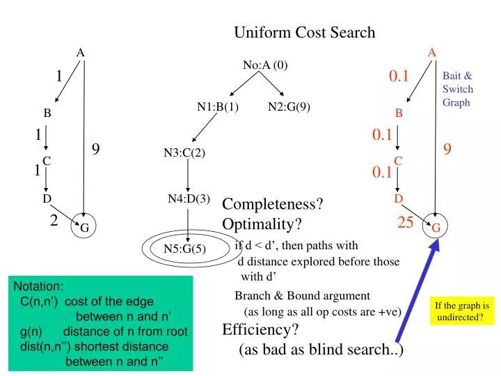
A. A. 1. 0.1. Bait & Switch Graph. N1:B(1). N2:G(9). B. B. 1. 0.1. 9. 9. N3:C(2). C. C. 1. 0.1. D. N4:D(3). D. 2. 25. G. G. N5:G(5). Uniform Cost Search. No:A (0). Completeness? Optimality? if d < d’, then paths with d distance explored before those

E N D
A A 1 0.1 Bait & Switch Graph N1:B(1) N2:G(9) B B 1 0.1 9 9 N3:C(2) C C 1 0.1 D N4:D(3) D 2 25 G G N5:G(5) Uniform Cost Search No:A (0) Completeness? Optimality? if d < d’, then paths with d distance explored before those with d’ Branch & Bound argument (as long as all op costs are +ve) Efficiency? (as bad as blind search..) Notation: C(n,n’) cost of the edge between n and n’ g(n) distance of n from root dist(n,n’’) shortest distance between n and n’’ If the graph is undirected?
N1:B(1) N2:G(9) N31:C(2) N41:D(3) N51:G(5) Uniform Cost Search on Undirected Graph A No:A (0) 1 B 1 • Cycles do not affect the • completeness and optimality! • The same world state may come • into the search queue multiple • times (e.g. N0:A; N32:A), but • each additional time it comes • it comes with a higher g-value! • If edge costs are positive then no single node can be expanded more than a finite times.. We will eventually get out of the cycles and find the optimal solution • You can reduce the number of Repeated expansions by doing cycle checking 9 N32:A(2) C 1 D N42:B(3) 2 G N52:C(3) Notation: C(n,n’) cost of the edge between n and n’ g(n) distance of n from root dist(n,n’’) shortest distance between n and n’’
Breadth-First goes level by level Visualizing Breadth-First & Uniform Cost Search This is also a proof of optimality…
Proof of Optimality of Uniform search Proof of optimality: Let N be the goal node we output. Suppose there is another goal node N’ We want to prove that g(N’) >= g(N) Suppose this is not true. i.e. g(N’) < g(N) --Assumption A1 When N was picked up for expansion, Either N’ itself, or some ancestor of N’, Say N’’ must have been on the search queue If we picked N instead of N’’ for expansion, It was because g(N) <= g(N’’) ---Fact f1 But g(N’) = g(N’’) + dist(N’’,N’) So g(N’) >= g(N’’) So from f1, we have g(N) <= g(N’) But this contradicts our assumption A1 No N’’ N N’ Holds only because dist(N’’,N’) >= 0 This will hold if every operator has +ve cost The partial path to N’ through N’’ is already longer than the path to N.
A 0.1 Bait & Switch Graph N1:B(.1) N2:G(9) B 0.1 9 N3:C(.2) C 0.1 N4:D(.3) D 25 G N5:G(25.3) Admissibility Informedness “Informing” Uniform search… No:A (0) Would be nice if we could tell that N2 is better than N1 --Need to take not just the distance until now, but also distance to goal --Computing true distance to goal is as hard as the full search --So, try “bounds” h(n) prioritize nodes in terms of f(n) = g(n) +h(n) two bounds: h1(n) <= h*(n) <= h2(n) Which guarantees optimality? --h1(n) <= h2(n) <= h*(n) Which is better function?
(if there are multiple goal nodes, we consider the distance to the nearest goal node) Several proofs: 1. Based on Branch and bound --g(N) is better than f(N’’) and f(n’’) <= cost of best path through N’’ 2. Based on contours -- f() contours are more goal directed than g() contours 3. Based on contradiction
Where do heuristics (bounds) come from? From relaxed problems (the more relaxed, the easier to compute heuristic, but the less accurate it is) For path planning on the plane (with obstacles)? For 8-puzzle problem? For Traveling sales person? Assume away obstacles. The distance will then be The straightline distance (see next slide for other abstractions) Assume ability to move the tile directly to the place distance= # misplaced tiles Assume ability to move only one position at a time distance = Sum of manhattan distances. Relax the “circuit” requirement. Minimum spanning tree
Different levels of abstraction for shortest path problems on the plane I The obstacles in the shortest path problem canbe abstracted in a variety of ways. --The more the abstraction, the cheaper it is to solve the problem in abstract space --The less the abstraction, the more “informed” the heuristic cost (i.e., the closer the abstract path length to actual path length) hD G “disappearing-act abstraction” I hC G “circular abstraction” hP I Actual h* Why are we inscribing the obstacles rather than circumscribing them? I G “Polygonal abstraction” G
How informed should the heuristic be? Total cost incurred in search Cost of computing the heuristic Cost of searching with the heuristic hC hD h0 h* hP • Not always clear where the total minimum occurs • Old wisdom was that the global min was closer to cheaper heuristics • Current insights are that it may well be far from the cheaper heuristics for many problems • E.g. Pattern databases for 8-puzzle • polygonal abstractions for SP • Plan graph heuristics for planning Reduced level of abstraction (i.e. more and more concrete)
h5 h4 h* Max(h2,h3) h1 h3 h2 Admissibility/Informedness Heuristic Value Seach Nodes
Performance on 15 Puzzle • Random 15 puzzle instances were first solved optimally using IDA* with Manhattan distance heuristic (Korf, 1985). • Optimal solution lengths average 53 moves. • 400 million nodes generated on average. • Average solution time is about 50 seconds on current machines.
Limitation of Manhattan Distance • To solve a 24-Puzzle instance, IDA* with Manhattan distance would take about 65,000 years on average. • Assumes that each tile moves independently • In fact, tiles interfere with each other. • Accounting for these interactions is the key to more accurate heuristic functions.
14 7 3 3 7 15 12 11 11 13 12 13 14 15 7 13 3 M.d. is 20 moves, but 28 moves are needed 12 7 15 3 11 11 14 12 13 14 15 12 11 3 M.d. is 17 moves, but 27 moves are needed 7 14 7 13 3 11 15 12 13 14 15 More Complex Tile Interactions Min disance (M.d.) is 19 moves, but 31 moves are needed.
Pattern Database Heuristics • Culberson and Schaeffer, 1996 • A pattern database is a complete set of such positions, with associated number of moves. • e.g. a 7-tile pattern database for the Fifteen Puzzle contains 519 million entries.
5 10 14 7 1 2 3 8 3 6 1 4 5 6 7 15 12 9 8 9 10 11 2 11 4 13 12 13 14 15 Heuristics from Pattern Databases 31 moves is a lower bound on the total number of moves needed to solve this particular state.
Precomputing Pattern Databases • Entire database is computed with one backward breadth-first search from goal. • All non-pattern tiles are indistinguishable, but all tile moves are counted. • The first time each state is encountered, the total number of moves made so far is stored. • Once computed, the same table is used for all problems with the same goal state.
The lower-bound (optimistic) estimate on the length of the path to N’ through N’’ is already longer than the path to N. Proof of Optimality of A* search Proof of optimality: Let N be the goal node we output. Suppose there is another goal node N’ We want to prove that g(N’) >= g(N) Suppose this is not true. i.e. g(N’) < g(N) --Assumption A1 When N was picked up for expansion, Either N’ itself, or some ancestor of N’, Say N’’ must have been on the search queue If we picked N instead of N’’ for expansion, It was because f(N) <= f(N’’) ---Fact f1 i.e. g(N) + h(N) <= g(N’’) + h(N’’) Since N is goal node, h(N) = 0 So, g(N) <= g(N’’) + h(N’’) But g(N’) = g(N’’) + dist(N’’,N’) Given h(N’) <= h*(N’’) = dist(N’’,N’) (lower bound) So g(N’) = g(N’’)+dist(N’’,N’) >= g(N’’) +h(N’’) ==Fact f2 So from f1 and f2 we have g(N) <= g(N’) But this contradicts our assumption A1 No f(n) is the estimate of the length of the shortest path to goal passing through n N’’ N N’ Holds only because h(N’’) is a lower bound on dist(N’’,N’)
Visualizing A* Search But, does f value really increase along a path? It will not expand Nodes with f >f* (f* is f-value of the Optimal goal which is the same as g* since h value is zero for goals) A* Uniform cost search
9 7 7 A .1 N1:B(.1+25.2) N1:B(.1+8.8) N2:G(9+0) N2:G(9+0) 8.8 20 25.2 B .1 9 N3:C(max(.2+0),8.8) 28 0 25.1 C .1 25 25 25 D N4:D(.3+25) 25 0 0 0 G This is just enforcing Triangle law of inequality That the sum of two sides Must be greater than the third B f(B)= .1+8.8 = 8.9 f(C)= .2+0 = 0.2 This doesn’t make sense since we are reducing the estimate of the actual cost of the path A—B—C—D—G To make f(.) monotonic along a path, we say f(n) = max( f(parent), g(n)+h(n)) C(B,C) 0.1 PathMax Adjustment C f(B) 8.9 f(C) 0.2 G A* Search—Admissibility, Monotonicity, Pathmax Correction Is magenta-h admissible? No:A (0) Is green-h admissible? Does f(c) make sense? No:A (0) Why wasn’t this needed for uniform cost search?
7 7 9 A .1 N1:B(.1+8.8) N1:B(.1+25.2) N2:G(9+0) N2:G(9+0) 20 8.8 25.2 B .1 9 N3:C(max(.2+0),8.8) 0 28 25.1 C .1 Consistency of a heuristic will be enforced if it obeys triangle inequality 25 25 25 D N4:D(.3+25) 25 0 0 0 G B f(B)= .1+8.8 = 8.9 f(C)= .2+0 = 0.2 This doesn’t make sense since we are reducing the estimate of the actual cost of the path A—B—C—D—G To make f(.) monotonic along a path, we say f(n) = max( f(parent), g(n)+h(n)) C(B,C) 0.1 PathMax Adjustment C h(B) 8.8 h(C) 0.1 G A* Search—Admissibility, Monotonicity, Pathmax Correction If a heuristic is inconsistently optimistic, then it can be more optimistic at a node than its parent node. When this happens, f values of the expanded nodes are not guaranteed to increase monotonically. Is magenta-h admissible? No:A (0) Is green-h admissible? Does f(c) make sense? No:A (0) Why wasn’t this needed for uniform cost search?
IDA*--do iterative depth first search but Set threshold in terms of f (not depth)
IDA* to handle the A* memory problem • Basicaly IDDFS, except instead of the iterations being defined in terms of depth, we define it in terms of f-value • Start with the f cutoff equal to the f-value of the root node • Loop • Generate and search all nodes whose f-values are less than or equal to current cutoff. • Use depth-first search to search the trees in the individual iterations • Keep track of the node N’ which has the smallest f-value that is still larger than the current cutoff. Let this f-value be next-largest-f-value -- If the search finds a goal node, terminate. If not, set cutoff = next-largest-f-value and go back to Loop Properties: Linear memory. #Iterations in the worst case? = Bd !! (Happens when all nodes have distinct f-values. There is such a thing as too much discrimination…)
Using memory more effectively: SMA* • A* can take exponential space in the worst case • IDA* takes linear space (in solution depth) always • If A* is consuming too much space, one can argue that IDA* is consuming too little • Better idea is to use all the memory that is available, and start cleaning up as memory starts filling up • Idea: When the memory is about to fill up, remove the leaf node with the worst f-value from the search tree • But remember its f-value at its parent (which is still in the search tree) • Since the parent is now the leaf node, it too can get removed to make space • If ever the rest of the tree starts looking less promising than the parent of the removed node, the parent will be picked up and expanded again. • Works quite well—but can thrash when memory is too low • Not unlike your computer with too little RAM..
On “predicting” the effectiveness of Heuristics Advanced Let us divide the number of nodes expanded nE into Two parts: nI which is the number of nodes expanded Whose f-values were strictly less than f* (I.e. the Cost of the optimal goal), and nG is the # of expanded Nodes with f-value greater than f*. So, nE=nI+nG A more informed heuristic is only guaranteed to have A smaller nI—all bets are off as far as the nG value is Concerned. In many cases nG may be relatively large Compared to nI making the nE wind up being higher For an informed heuristic! • Unfortunately, it is not the case that a heuristic h1 that is more informed than h2 will always do fewer node expansions than h2. -We can only gurantee that h1 will expand less nodes with f-value less than f* than h2 will • Consider the plot on the right… do you think h1 or h2 is likely to do better in actual search? • The “differentiation” ability of the heuristic—I.e., the ability to tell good nodes from the bad ones-- is also important. But it is harder to measure. • Some new work that does a histogram characterization of the distribution of heuristic values [Korf, 2000] • Nevertheless, informedness of heuristics is a reasonable qualitative measure h* h1 Heuristic value h2 Is h1 better or h2? Nodes
Not enough to show the correct configuration of the 18-puzzle problem or rubik’s cube.. (although by including the list of actions as part of the state, you can support hill-climbing)
What is needed: --A neighborhood function The larger the neighborhood you consider, the less myopic the search (but the more costly each iteration) --A “goodness” function needs to give a value to non-solution configurations too for 8 queens: (-ve) of number of pair-wise conflicts
Problematic scenarios for hill-climbing Solution(s): Random restart hill-climbing Do the non-greedy thing with some probability p>0 Use simulated annealing Ridges • When the state-space landscape has local minima, any search that moves only in the greedy direction cannot be (asymptotically) complete • Random walk, on the other hand, is asymptotically complete Idea: Put random walk into greedy hill-climbing
Making Hill-Climbing Asymptotically Complete • Random restart hill-climbing • Keep some bound B. When you made more than B moves, reset the search with a new random initial seed. Start again. • Getting random new seed in an implicit search space is non-trivial! • In 8-puzzle, if you generate a random state by making random moves from current state, you are still not truly random (as you will continue to be in one of the two components) • “biased random walk”: Avoid being greedy when choosing the seed for next iteration • With probability p, choose the best child; but with probability (1-p) choose one of the children randomly • Use simulated annealing • Similar to the previous idea—the probability p itself is increased asymptotically to one (so you are more likely to tolerate a non-greedy move in the beginning than towards the end) With random restart or the biased random walk strategies, we can solve very large problems million queen problems in under minutes!