Download
1 / 60
600 likes | 742 Views
The Cosmic History of Element Formation. Wolfgang Hillebrandt, MPI für Astrophysik Lecture, Graduiertenkolleg GRK1147, January 23, 2014. Outline: Introduction Abundance determinations Galactic chemical evolution Type Ia supernovae: an example. 0. Introduction.

E N D
The Cosmic History of Element Formation Wolfgang Hillebrandt, MPI für Astrophysik Lecture, Graduiertenkolleg GRK1147, January 23, 2014 Outline: Introduction Abundance determinations Galactic chemical evolution Type Ia supernovae: an example
… and what we have today What the big bang made… Compositional Evolution of the Universe
… and what we have today What the big bang made… Compositional Evolution of the Universe When, and how did metal enrichment happen??
THE ISOTOPIC LANDSCAPE AND COSMIC SOURCES Mass known Half-life known s process nothing known p process r process rp process Supernovae stellar burning Cosmic Rays Big Bang Pb (82) Sn (50) • ~300 Stable and ~2400 radioactive isotopes • Cosmic nucleosynthesis proceeds over much of this range • Knowledge of nuclear physics is incomplete • Figure courtesy Hendrik Schatz Fe (26) protons H(1) neutrons
1. Abundance Determinations Anders & Grevesse (1989)
Oscillator modeling • – oscillator strength • – natural width • – pressure broadening • – Doppler broadening • • Line strength often described • by equivalent width • Simple approach: Abundance determination from “curve of growth”: • W: equivalent width • f: oscillator strength • (example: for the sun) StEllar spectra - Spectral synthesis
Its not sufficient to consider only one line; one has to take more lines into account • Detailed problem is complex; theoretical uncertainties and difficulties StEllar spectra - Spectral synthesis
Whole spectrum is calculated from a model atmosphere • Simultaneous determination of effective temperature, gravity, and abundances StEllar spectra - Spectral synthesis Resulting abundance ratio: [Fe/H] ≈ -3.1 (Sneden et al., 1996)
“Bracket notation”: [i/j] := log(Xi/Xj)/log(Xi/Xj)๏ i.e.: [Fe/H] = log{(XFe/XH)/(XFe /XH)๏}
Stars in the solar neighbourhood Results - A few examples Nomoto et al. (2006) (blue lines: model “predictions”)
Light-element abundances in • halo stars Results - A few examples Kraft et al. (1997) M 13 Very non-solar! ๏ Caretta et al. (2009)
Galactic abundance gradients (stars and ISM) Results - A few examples Abundances vary with galactocentric radius! Chiappini et al. (2001) (red dot: sun; solid lines: models)
memories of first stellar/SN nucleosynthesis • rare: • 2 stars at [Fe/H]<-5 • need high-resolution spectrographs and large surveys OBSERVATIONS OF EARLY-GENERATION STARS Time since Big Bang [Fe/H]=0 [Fe/H]=-4 [Fe/H]=-5 [Fe/H]=-∞
OBSERVATIONS OF EARLY-GENERATION STARS Rare earth abundances in r-rich halo stars and solar-system r- only abundances (Arlandini et al. (1999) and Simmerer et al. (2004)) (normalized at Eu). Sneden et al. (2009)
SMM/SN1987A 56Ni decay • in-situ measurement of nucleosynthesis ejecta in (current-Universe) sources • more detail accessible • test the models OBSERVATIONS OF EJECTA FROM NUCLEOSYNTHESIS SOURCES 26Al Puppis A/XMM O Ne Mg Si 60Fe
Chondrites: contain tiny rounded bodies (chondrules) • Achondrites: quite different in composition and structure, resembling terrestrial material • Carbonaceous chondrites: • Primitive chondrites • Most representative abundances chondrite Meteorites – Solar-System Isotopic abundances achondrite iron • Chemical composition can be measured with extraordinary high accuracy (mass spectrometry) • Seem to be representative of solar system matter • But: no information about other stars!
Solar system element/isotope abundances are well determined (solar spectrum, cc-chondrites):How `typical‘ is the sun (CNO, iron)? Conflict with helioseismology (Asplund et al.)? • Isotopic abundances (other than solar) are known in a few rare cases only (requires high-quality high-resolution spectra) • Abundances in stars (and the ISM) show a lot of scatter (metallicity, `abundance gradients‘, different populations, `anomalies‘): Is this, in part, a problem of the abundance determinations (spectra quality and modeling)? Or is there a physical reason we can understand? Summary – Part 1
GCE tries to understand the evolution of the chemical composition of the Universe based on our knowledge on the contributions of the individual NS sites, and on the evolution of cosmic structure. • GCE is linked to many subjects: • – all phases of stellar evolution • – galactic dynamics and evolution • – cosmology 2. Galactic chemical evolution (GCE) Woosley, Heger & Weaver (2002)
1. Start from a gas cloud already present at t=0 (monolithic model). No flows allowed (closed-box) or, alternatively, assume that the gas accumulates either fast or slowly and the system has outflows (open model) 2. Assume that the gas at t=0 is primordial (no metals) or, alternatively, assume that the gas at t=0 is pre-enriched by Pop III stars Initial Conditions
The most common parametrization is the Schmidt (1959) law where the SFR is proportional to some power (k=2) of the gas density Kennicutt (1998) suggested k=1.5 from studying star forming galaxies, but also a law depending of the rotation angular speed of gas Other parameters such as gas temperature, viscosity and magnetic field are usually ignored Parametrization of the SFR
SF induced by spiral density waves (Wyse & Silk, 1998; Prantzos, 2002) SF accounting for feedback (Dopita & Ryder, 1974) Other Parametrizations of the SFR SFR = aV(R)R -1σgas1.5 SFR = νσtotk1σgask2
Distribution of stellar masses at birth. Definitions: – number fraction of stars formed per interval [m,m+dm] = Φ(m) – mass fraction of stars formed ... mΦ(m) = ξ (m) normalisation: min, max are minimum and maximum stellar masses • Observations: star counts in the local region (take into account the life time of the stars), star counts in starforming regions. • Analytic approximations: (piecewise) powerlaws. The simplest case is the Salpeter IMF: • Uncertainties: no detailed understanding of SF process yet, IMF at low metallicity Initial mass function
During their evolution and at their death, stars release processed matter. The NS products (yields) depend on stellar mass and composition. CE requires detailed knowledge of stellar life times and NS yields. Stellar Yields
Stellar Yields Woosley, Heger & Weaver (2002)
Stellar Yields Woosley, Heger & Weaver (2002)
Mass ejection Assumption: all matter is ejected in a single event (i.e. on a timescale negligible compared to the galactic evolution timescales) and mixed into the (local) gas (“instantaneous recycling”): Ri(t,m) = δ(t-τ(m))Ri(m)
One-zone models: • perfect mixing in the homogeneous • physical domain • – closed box models • – open box models: some • prescription of infall and outflows • Multizone models: • coupled open box models with • interzone mass transfer • Chemodynamical models: • (multidimensional) selfconsistent • treatment of the entire • galaxy with all/some of the • components and interactions • described above. Chemical evolution models
Assume homogeneity in the physical domain (galaxy,...) due to fast mixing, neglect spatial derivatives and therefore large-scale • coupling ==> equations for the integral quantities gas mass and • stellar mass, and for the (spatially constant) abundances, • star formation rates, ... • Boundaries closed (the “simple model”) or open (replenishment of the gas by infall of (primordial?) matter, outflow of processed gas). • Initial conditions: no stars, only gas with primordial composition. • Allows to understand basic effects like the age-metallicity • relation and the distribution of stars with metallicity. One-Zone model in more detail
How Do the Models Perform? Solar neighbor-hood (Prantzos, 2011) Metallicity distribution of G-type stars • Solar neighborhood looks OK
Time progesses from ‘blue’ to ‘red’. How the Models Perform? Chiappini et al. (2001) • Abundance gradients look OK (inhomogenous models)
But: galactic elemental composition NOT consistently reproduced How Does Our Model Perform?
How the Model Perform? Francois et al. (2004)
How the Model Perform? Francois et al. (2004)
How the Model Perform? Francois et al. (2004)
Are the stellar Yields wrong (SN Ia)? Francois et al. (2004)
Other Galaxies: SN Ia vs. SN II • dSph Galaxies in Local Group
GCE models are able to reproduce the evolution of many GCE parameters in the Milky Way and other galaxies, such as abundance patterns (as well as starformation rates and stellar populations) reasonably well. • But, despite of rather many (free) parameters, there are several problems still (N, Co, ...): Limited data sets? Stellar astrophysics? Cosmological model (initial data, ...)? • Goal: models with more `predictive power‘: Chemo-dynamical models. Summary – Part 2
Simulate the dynamical & chemical evolution • of a galaxy selfconsistently, tracing a limited • number of species. • Initial conditions: • – parametrisation of an early state of the • galaxy (from a cosmological simulation of the • evolution of largescale structure starting at • high redshift). • Comparison with observations by determination of • – the morphological and kinematic structure • – the starformation rate and the rates for PN, SN • – the distribution of elements over the galaxy • – the stellar populations (==> synthetic spectra) Chemo-dynamical models
THE ‘ZOO’ OF (POSSIBLE) THERMONUCLEAR EXPLOSIONS • ‘Single degenerates’ • ● Chandrasekhar mass • - Pure deflagration • - ‘delayed’ detonation • ● sub-Chandrasekhar mass • ‘Double degenerates’ • ● C/O + C/O • ● C/O + He • Which of them are realized in Nature? All of them?
HOW MUCH DO DIFFERENT CHANNELS CONTRIBUTE TO THE RATE? Ruiter et al. (2011)
Nucleosynthesis in SN Ia Tycho‘s supernova (SN 1572) X-ray spectrum (Badenes et al. 2006): M(Fe) ≈ 0.74M๏
(Single-denerate MChan with parametrized burning speed) “W7” - an example .... Iwamoto et al. (1999)
56Nib30= 0.44M๏56NiW7 = 0.63M๏ .... Or a “pure-deflagration” model Travaglio et al. (2004)
“Abundance tomography” – reconstructed abundances SN 2002bo (Stehle et al., 2005)